| |
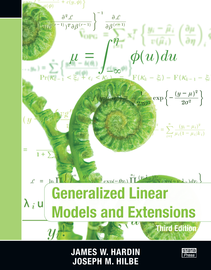
Contents of Generalized Linear Models and Extensions, Third Edition
by James W. Hardin and Joseph M. Hilbe

Generalized linear models (GLMs) extend linear regression to models
with a non-Gaussian, or even discrete, response. GLM theory is
predicated on the exponential family of distributions—a class so rich
that it includes the commonly used logit, probit, and Poisson models.
Although one can fit these models in Stata by using specialized
commands (for example, logit for logit models), fitting them as GLMs
with Stata’s glm command offers some advantages. For example, model
diagnostics may be calculated and interpreted similarly regardless of
the assumed distribution.
This text thoroughly
covers GLMs, both theoretically and computationally, with an emphasis
on Stata. The theory consists of showing how the various GLMs are
special cases of the exponential family, showing general properties of
this family of distributions, and showing the derivation of maximum
likelihood (ML) estimators and standard errors. Hardin and Hilbe show
how iteratively reweighted least squares, another method of parameter
estimation, are a consequence of ML estimation using Fisher scoring.
The authors also discuss different methods of estimating standard
errors, including robust methods, robust methods with clustering,
Newey–West, outer product of the gradient, bootstrap, and jackknife.
The thorough coverage of model diagnostics includes measures of
influence such as Cook’s distance, several forms of residuals, the
Akaike and Bayesian information criteria, and various R2-type measures
of explained variability.
After presenting general
theory, Hardin and Hilbe then break down each distribution. Each
distribution has its own chapter that explains the computational
details of applying the general theory to that particular distribution.
Pseudocode plays a valuable role here, because it lets the authors
describe computational algorithms relatively simply. Devoting an entire
chapter to each distribution (or family, in GLM terms) also allows for
the inclusion of real-data examples showing how Stata fits such models,
as well as presenting certain diagnostics and analytical strategies
that are unique to that family. The chapters on binary data and on
count (Poisson) data are excellent in this regard. Hardin and Hilbe
give ample attention to the problems of overdispersion and zero
inflation in count-data models.
The final part of the
text concerns extensions of GLMs, which come in three forms. First, the
authors cover multinomial responses, both ordered and unordered.
Although multinomial responses are not strictly a part of GLM, the
theory is similar in that one can think of a multinomial response as an
extension of a binary response. The examples presented in these
chapters often use the authors’ own Stata programs, augmenting official
Stata’s capabilities. Second, GLMs may be extended to clustered data
through generalized estimating equations (GEEs), and one chapter covers
GEE theory and examples. Finally, GLMs may be extended by programming
one’s own family and link functions for use with Stata’s official glm
command, and the authors detail this process.
In addition to other
enhancements—for example, a new section on marginal effects—the third
edition contains several new extended GLMs, giving Stata users new ways
to capture the complexity of count data. New count models include a
three-parameter negative binomial known as NB-P, Poisson inverse
Gaussian (PIG), zero-inflated generalized Poisson (ZIGP), a rewritten
generalized Poisson, two- and three-component finite mixture models,
and a generalized censored Poisson and negative binomial. This edition
has a new chapter on simulation and data synthesis, but also shows how
to construct a wide variety of synthetic and Monte Carlo models
throughout the book.
Table of Contents
List of Tables
List of Figures
Preface
- Introduction
- Origins and motivation
- Notational conventions
- Applied or theoretical?
- Road map
- Installing the support materials
I Foundations of Generalized Linear Models
- Generalized Linear Models
- Components
- Assumptions
- Exponential family
- Example: Using an offset in a GLM
- Summary
- GLM estimation algorithms
- Newton–Raphson (using the observed Hessian)
- Starting values for Newton–Raphson
- IRLS (using the expected Hessian)
- Starting values for IRLS
- Goodness of fit
- Estimated variance matrices
- Hessian
- Outer product of the gradient
- Sandwich
- Modified sandwich
- Unbiased sandwich
- Modified unbiased sandwich
- Weighted sandwich: Newey-West
- Jackknife
- Usual jackknife
- One-step jackknife
- Weighted jackknife
- Variable jackknife
- Bootstrap
- Usual bootstrap
- Grouped bootstrap
- Estimation algorithms
- Summary
- Analysis of fit
- Deviance
- Diagnostics
- Cook's distance
- Overdispersion
- Assessing the link function
- Residual analysis
- Response residuals
- Working residuals
- Pearson residuals
- Partial residuals
- Anscombe residuals
- Deviance residuals
- Adjusted deviance residuals
- Likelihood residuals
- Score residuals
- Checks for systematic departure from the model
- Model statistics
- Criterion measures
- AIC
- BIC
- The interpretation of R2 in linear regression
- Percent variance explained
- The ratio of variances
- A transformation of the likelihood ratio
- A transformation of the F test
- Squared correlation
- Generalizations of linear regression R2 interpretations
- Efron's pseudo-R2
- McFadden's likelihood-ratio index
- Ben-Akiva and Lerman adjusted likelihood-ratio index
- McKelvey and Zavoina ratio of variances
- Transformation of likelihood ratio
- Cragg and Uhler normed measure
- More R2 measures
- The count R2
- The adjusted count R2
- Veall and Zimmermann R2
- Cameron–Windmeijer R2
- Marginal effects
- Marginal effects for GLMs
- Discrete change for GLMs
- Data Synthesis
- Generating correlated data
- Generating data from a specified population
- Generating data for linear regression
- Generating data for logistic regression
- Generating data for probit regression
- Generating data for cloglog regression
- Generating data for Gaussian variance and log link
- Generating underdispersed count data
- Simulation
- Heteroskedasticity in linear regression
- Power analysis
- Comparing fit of Poisson and negative binomial
- Effect of omitted covariate on R2Efron in Poisson regression
II Continuous Response Models
- The Gaussian family
- Derivation of the GLM Gaussian family
- Derivation in terms of the mean
- IRLS GLM algorithm (nonbinomial)
- ML estimation
- GLM log-normal models
- Expected versus observed information matrix
- Other Gaussian links
- Example: Relation to OLS
- Example: Beta-carotene
- The gamma family
- Derivation of the gamma model
- Example: Reciprocal link
- Maximum likelihood estimation
- Log-gamma models
- Identity-gamma models
- Using the gamma model for survival analysis
- The inverse Gaussian family
- Derivation of the inverse Gaussian model
- The inverse Gaussian algorithm
- Maximum likelihood algorithm
- Example: The canonical inverse Gaussian
- Non-canonical links
- The power family and link
- Power links
- Example: Power link
- The power family
III Binomial Response Models
- The binomial-logit family
- Derivation of the binomial model
- Derivation of the Bernoulli model
- The binomial regression algorithm
- Example: Logistic regression
- Model producing logistic coefficients: The heart data
- Model producing logistic odds ratios
- GOF statistics
- Interpretation of parameter estimates
- The general binomial family
- Non-canonical binomial models
- Non-canonical binomial links (binary form)
- The probit model
- The clog-log and log-log models
- Other links
- Interpretation of coefficients
- Identity link
- Logit link
- Log link
- Log complement link
- Summary
- Generalized binomial regression
- The problem of overdispersion
- Overdispersion
- Scaling of standard errors
- Williams' procedure
- Robust standard errors
IV Count Response Models
- The Poisson family
- Count response regression models
- Derivation of the Poisson algorithm
- Poisson regression: Examples
- Example: Testing overdispersion in the Poisson model
- Using the Poisson model for survival analysis
- Using offsets to compare models
- Interpretation of coefficients
- The negative binomial family
- Constant overdispersion
- Variable overdispersion
- Derivation in terms of a Poisson–gamma mixture
- Derivation in terms of the negative binomial probability function
- The canonical link negative binomial parameterization
- The log-negative binomial parameterization
- Negative binomial examples
- The geometric family
- Interpretation of coefficients
- Other count data models
- Count response regression models
- Zero-truncated models
- Zero-inflated models
- Hurdle models
- Negative binomial(P) models
- Heterogeneous negative binomial models
- Generalized Poisson regression models
- Poisson inverse Gaussian models
- Censored count response models
- Finite mixture models
V Multinomial Response Models
- The ordered response family
- Interpretation of coefficients: Single binary predictor
- Ordered outcomes for general link
- Ordered outcomes for specific links
- Ordered logit
- Ordered probit
- Ordered clog-log
- Ordered log-log
- Ordered cauchit
- Generalized ordered outcome models
- Example: Synthetic data
- Example: Automobile data
- Partial proportional-odds models
- Continuation ratio models
- Unordered response family
- The multinomial logit model
-
- Interpretation of coefficients: Single binary predictor
- Example: Relation to logistic regression
- Example: Relation to conditional logistic regression
- Example: Extensions with conditional logistic regression
- The independence of irrelevant alternatives
- Example: Assessing the IIA
- Interpreting coefficients
- Example: Medical admissions—introduction
- Example: Medical admissions—summary
- The multinomial probit model
- Example: A comparison of the models
- Example: Comparing probit and multinomial probit
- Example: Concluding remarks
VI Extensions to the GLM
- Extending the likelihood
- The quasi-likelihood
- Example: Wedderburn's leaf blotch data
- Generalized additive models
- Clustered data
- Generalization from individual to clustered data
- Pooled estimators
- Fixed effects
- Unconditional fixed-effects estimators
- Conditional fixed-effects estimators
- Random effects
- Maximum likelihood estimation
- Gibbs sampling
-
- GEEs
- Other models
VII Stata Software
- Programs for Stata
- The glm command
- Syntax
- Description
- Options
- The predict command after glm
- Syntax
- Options
- User-written programs
- Global macros available for user-written programs
- User-written variance functions
- User-written programs for link functions
- User-written programs for Newey-West weights
- Remarks
- Equivalent commands
- Special comments on family(Gaussian) models
- Special comments on family(binomial) models
- Special comments on family(nbinomial) models
- Special comment on family(gamma) link(log) models
A Tables
References
Author index
Subject index
© Copyright StataCorp LP 2002-2015.


|
|


