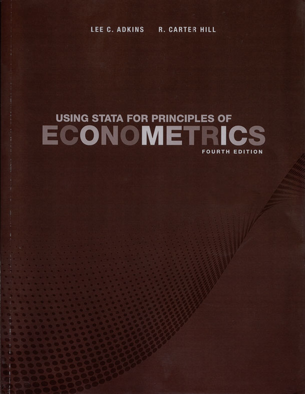
Using Stata for Principles of Econometrics, 3rd Edition
by Lee C. Adkins and R. Carter Hill
 Using
Stata for Principles of Econometrics, Fourth Edition, by Lee C. Adkins
and R. Carter Hill, is a companion to the introductory econometrics
textbook Principles of Econometrics, Fourth Edition. Together, the two
books provide a very good introduction to econometrics for
undergraduate students and first-year graduate students. Using
Stata for Principles of Econometrics, Fourth Edition, by Lee C. Adkins
and R. Carter Hill, is a companion to the introductory econometrics
textbook Principles of Econometrics, Fourth Edition. Together, the two
books provide a very good introduction to econometrics for
undergraduate students and first-year graduate students.
The main textbook takes a learn-by-doing approach to econometric
analysis, and this companion book illustrates the "doing" part using
Stata. Adkins and Hill briefly show how to use Stata's menu system and
command line before delving into their many examples.
Using Stata for Principles of Econometrics, Fourth Edition shows how to
use Stata to reproduce the examples in the main textbook and how to
interpret the output. The current edition has been updated to include
features introduced in Stata 11, such as the margins command to compute
elasticities. Together with Principles of Econometrics, Fourth Edition,
the reader will not only learn econometrics but also gain the
confidence needed to perform his or her own work using Stata.
Table of contents Chapter 1 Introducing Stata
- 1.1 Starting Stata
1.2 The opening display
1.3 Exiting Stata
1.4 Stata data files for Principles of Econometrics
1.4.1 A working directory
1.5 Opening Stata data files
1.5.1 The use command
1.5.2 Using the toolbar
1.5.3 Using files on the Internet
1.5.4 Locating book files on the Internet
1.6 The variables window
-
1.6.1 Using the data editor for a single label
1.6.2 Using the data utility for a single label
1.6.3 Using variables manager
1.7 Describing the data and obtaining summary statistics
1.8 The Stata help system
1.8.1 Using keyword search
1.8.2 Using command search
1.8.3 Opening a dialog box
-
1.8.4 Complete documentation in Stata manuals
1.9 Stata commands syntax
1.9.1 Syntax of summarize
1.9.2 Learning syntax using the review window
1.10 Saving your work
1.10.1 Copying and pasting
1.10.2 Using a log file
1.11 Using the data browser
1.12 Using Stata graphics
1.12.1 Histograms
1.12.2 Scatter diagrams
1.13 Using Stata do-files
1.14 Creating and managing variables
1.14.1 Creating (generating) new variables
1.14.2 Using the expression builder
1.14.3 Dropping or renaming a variable
1.14.3 Using arithmetic operators
1.14.5 Using Stata math functions
1.15 Using Stata density functions
1.15.1 Cumulative distribution functions
1.15.2 Inverse cumulative distribution functions
1.16 Using and displaying scalars
1.16.1 Example of standard normal cdf
1.16.2 Example of t-distribution tail-cdf
1.16.3 Example of computing percentile of the standard normal
1.16.4 Example of computing percentile of the t-distribution
- 1.17 A scalar dialog box
- 1.18 Using factor variables
1.18.1 Creating indicator variables using a logical operator
1.18.2 Creating indicator variables using tabulate
Key terms
Chapter 1 Do-file
Chapter 2 Simple linear regression
- 2.1 The flood expenditure data
2.1.1 Starting a new problem
2.1.2 Starting a log file
2.1.3 Opening a Stata data file
2.1.4 Browsing and listing the data
2.2 Computing summary statistics
2.3 Creating a scatter diagram
2.3.1 Enhancing the plot
2.4 Regression
2.4.1 Fitted values and residuals
2.4.2 Computing an elasticity
2.4.3 Plotting the fitted regression line
2.4.4 Estimating the variance of the error term
2.4.5 Viewing estimated variances and covariances
2.5 Using Stata to obtain predicted values
2.6 Estimating nonlinear relationships
2.6.1 A quadratic model
2.6.2 A log-linear model
2.7 Regression with indicator variables
Appendix 2A Average marginal effects
2A.1 Elasticity in a linear relationship
2A.2 Elasticity in a quadratic relationship
2A.3 Slope in a log-linear model
Appendix 2B A simulation experiment
Key terms
Chapter 2 do-file Chapter 3 Interval Estimation and Hypotheses Testing
- 3.1 Interval estimates
3.1.1 Critical values from the t-distribution
3.1.2 Creating an interval estimate
3.2 Hypothesis tests
3.2.1 Right tail test of significance
3.2.2 Right tail test of an economic hypothesis
3.2.3 Left tail test of an economic hypothesis
3.2.4 Two tail test of an economic hypothesis
3.3 P-values
3.3.1 P-value test of a right tail test
3.3.2 P-value test of a left tail test
3.3.3 P-value test of a two tail test
3.3.4 P-values in Stata output - 3.3.5 Testing and estimating linear combinations of parameters
- Appendix 3A Graphical tools
Appendix 3B Monte Carlo simulation
Key terms
Chapter 3 Do-file
Chapter 4 Prediction, Goodness-of-Fit and Modeling Issues
4.1 Least squares prediction
4.1.1 Editing the data
4.1.2 Estimate the regression and obtain post-estimation results
4.1.3 Creating the prediction interval
4.2 Measuring goodness-of-fit
4.2.1 Correlations and R^2
4.3 The effects of scaling and transforming the data
4.3.1 The reciprocal functional form
4.3.2 Plotting the fitted linear-log model
4.3.3 Editing graphs
4.4 Analyzing the residuals
4.4.1 The Jarque-Bera test
4.4.2 Chi-square distribution critical values
4.4.3 Chi-square distribution p-values
4.5 Polynomial models
4.5.1 Estimating and checking the linear relationship
4.5.2 Estimating and checking a cubic equation
4.5.3 Estimating a log-linear yield growth model
4.6 Estimating a log-linear wage equation
4.6.1 The log-linear model
4.6.2 Calculating wage predictions
4.6.3 Constructing wage plots
4.6.4 Generalized R2
4.6.5 Prediction intervals in the log-linear model
4.7 A log-log model
Key Terms
Chapter 4 Do-file
Chapter 5 Multiple Linear Regression
- 5.1 Big Andy’s Burger Barn
5.2 Least squares prediction
5.3 Sampling precision
5.4 Confidence intervals
5.4.1 Confidence interval for a linear combination of parameters
5.5 Hypothesis tests
5.5.1 Two-sided tests
5.5.2 One-sided tests
5.5.3 Testing a linear combination
5.6 Polynomial equations
5.6.1 Optimal advertising: nonlinear combinations of parameters
5.6.2 Using factor variables for interactions
5.7 Interactions
5.8 Goodness-of-fit
Key terms
Chapter 5 do-file
Chapter 6 Further Inference in the Multiple Regression Model
- 6.1 The F-test
6.1.1 Testing the significance of the model
6.1.2 Relationship between t- and F-tests
6.1.3 More general F-tests
6.2 Nonsample information
6.3 Model specification
6.3.1 Omitted variables
6.3.2 Irrelevant variables
6.3.3 Choosing the model
6.4 Poor data, collinearity, and insignificance
Key terms
Chapter 6 do-file
Chapter 7 Using Indicator Variables
- 7.1 Indicator variables
7.1.1 Creating indicator variables
7.1.2 Estimating an indicator variable regression
7.1.3 Testing the significance of the indicator variables
7.1.4 Futher calculations
7.1.5 Computing average marginal effects
7.2 Applying indicator variables
7.2.1 Interactions between qualitative factors
7.2.2 Adding regional indicators
7.2.3 Testing the equivalence of two regressions
7.2.4 Estimating separate regressions
7.2.5 Indicator variables in log-linear models
7.3 The linear probability model
7.4 Treatment effects
7.5 Differences-in-differences estimation
Key terms
Chapter 7 do-file
Chapter 8 Heteroskedasticity
8.1 The nature of heteroskedasticity
8.2 Detecting heteroskedasticity
8.2.1 Residual plots
8.2.2 Lagrange multiplier tests
8.2.3 The Goldfeld-Quandt test
8.3 Heteroskedastic-consistent standard errors
8.4 The generalized least squares estimator
8.4.1 GLS using grouped data
8.4.2 Feasible GLS–a more general case
8.5 Heteroskedasticity in the linear probability model
Key terms
Chapter 8 do-file Chapter 9 Regression with Time-Series Data: Stationary Variables
9.1 Introduction
9.1.1 Defining time-series in Stata
9.1.2 Time-series plots
9.1.3 Stata's lag and difference operators
9.2 Finite distributed lags
9.3 Serial correlation
9.4 Other tests for serial correlation
9.5 Estimation with serially correlated errors
9.5.1 Least squares and HAC standard errors
9.5.2 Nonlinear least squares
9.5.3 A more general model
9.6 Autoregressive distributed lag models
9.6.1 Phillips curve
9.6.2 Okun's law
9.6.3 Autoregressive models
9.7 Forecasting
9.7.1 Forecasting with an AR model
9.7.2 Exponential smoothing
9.8 Multiplier analysis
9.9 Appendix
9.9.1 Durbin-Watson test
9.9.2 Prais-Winsten FGLS
Key terms
Chapter 9 do-file Chapter 10 Random Regressors and Moment Based Estimation
- 10.1 Least squares estimation of a wage equation
10.2 Two-stage least squares
10.3 IV estimation with surplus instruments
10.3.1 Illustrating partial correlations
10.4 The Hausman test for endogeneity
10.5 Testing the validity of surplus instruments
10.6 Testing for weak instruments
10.7 Calculating the Cragg-Donald F-statistic
10.8 A simulation experiment
Key terms
Chapter 10 do-file
Chapter 11 Simultaneous Equations Models
- 11.1 Truffle supply and demand
11.2 Estimating the reduced form equations
11.3 2SLS estimates of truffle demand
11.4 2SLS estimates of truffle supply
11.5 Supply and demand of fish
11.6 Reduced forms for fish price and quantity
11.7 2SLS estimates of fish demand
11.8 2SLS alternatives
11.9 Monte Carlo simulation
Key terms
Chapter 11 do-file
Chapter 12 Nonstationary Time Series Data and Cointegration
12.1 Stationary and nonstationary data
12.1.1 Review: generating dates in Stata
12.1.2 Extracting dates
12.1.3 Graphing the data
12.2 Spurious regressions
12.3 Unit root tests for stationarity
12.4 Integration and cointegration
12.4.1 Engle-Granger test
12.4.2 Error-correction model
Key terms
Chapter 12 do-file
Chapter 13 Vector Error Correction and Vector Autoregressive Models
13.1 VEC and VAR models
13.2 Estimating a VEC model
13.3 Estimating a VAR
13.4 Impulse responses and variance decompositions
Key Terms
Chapter 13 Do-file
Chapter 14 Time-Varying Volatility and ARCH Models
14.1 ARCH model and time-varying volatility
14.2 Testing, estimating, and forecasting
14.3 Extensions
14.3.1 GARCH
14.3.2 Threshold GARCH
14.3.3 GARCH-in-mean
Key Terms
Chapter 14 Do-file
Chapter 15 Panel Data models
15.1 A microeconomic panel
15.2 A pooled model
15.2.1 Cluster-robust standard errors
15.3 The fixed effects model
15.3.1 The fixed effects estimator
15.3.2 The fixed effects estimator using xtreg
15.3.3 Fixed effects using the complete panel
15.4 Random effects estimation
15.4.1 The GLS transformation
15.4.2 The Breusch-Pagan test
15.4.3 The Hausman test
15.4.4 The Hausman-Taylor model
15.5 Sets of regression equations
15.5.1 Seemingly unrelated regressions
15.5.2 SUR with wide data
15.6 Mixed models
Key terms
Chapter 15 do-file
Chapter 16 Qualitative and Limited Dependent Variable Models
16.1 Models with binary dependent variables
16.1.1 Average marginal effects
16.1.2 Probit marginal effects: details
16.1.3 Standard error of average marginal effect
16.2 The logit model for binary choice
16.2.1 Wald tests
16.2.2 Likelihood ratio tests
16.2.3 Logit estimation
16.2.4 Out-of-sample prediction
16.3 Multinomial logit
16.4 Conditional logit
16.4.1 Estimation using asclogit
16.5 Ordered choice models
16.6 Models for count data
16.7 Censored data models
16.7.1 Simulated data example
16.7.2 Mroz data example
16.8 Selection bias
Key terms
Chapter 16 do-file
A.1 Stata math and logical operators
A.2 Math functions
A.3 Extensions to generate
A.4 The calculator
A.5 Scientific notation
A.6 Numerical derivatives and integrals
Key terms
Appendix A do-file
Appendix B Review of Probability
B.1 Stata probability functions
B.2 Binomial distribution
B.3 Normal distribution
B.3.1 Normal density plots
B.3.2 Normal probability calculations
B.4 Student's t-distribution
B.4.1 Plot of standard normal and t(3)
B.4.2 t-distribution probabilities
B.4.3 Graphing tail probabilities
B.5 F-distribution
B.5.1 Plotting the F-density
B.5.2 F-distribution probability calculations
B.6 Chi-square distribution
B.6.1 Plotting the chi-square density
B.6.2 Chi-square probability calculations
B.7 Random numbers
B.7.1 Using inversion method
B.7.2 Creating uniform random numbers
Key terms
Appendix B do-file
Appendix C Review of Statistical Inference
C.1 Examining the hip data
C.1.1 Constructing a histogram
C.1.2 Obtaining summary statistics
C.1.3 Estimating the population mean
C.2 Using simulated data values
C.3 The central limit theorem
C.4 Interval estimation
C.4.1 Using simulated data
C.4.2 Using the hip data
C.5 Testing the mean of a normal population
C.5.1 Right rail test
C.5.2 Two tail test
C.6 Testing the variance of a normal population
C.7 Testing the equality of two normal population means
C.7.1 Population variances are equal
C.7.2 Population variances are unequal
C.8 Testing the equality of two normal population variances
C.9 Testing normality
C.10 Maximum likelihood estimation
C.11 Kernel density estimator
Key Terms
Appendix C Do-file
Index
© Copyright StataCorp LP 1996-2015.


|


