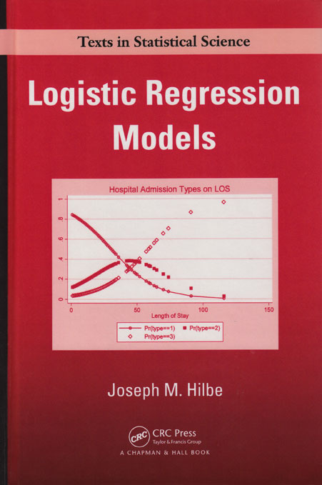
Logistic Regression Models

by Joseph M. Hilbe

  Logistic Regression Models, by Joseph Hilbe, arose from Hilbe’s course in logistic regression at statistics.com. The book includes many Stata examples using both official and user-written commands and includes Stata output and graphs.

Hilbe begins with simple contingency tables and covers fitting algorithms, parameter interpretation, and diagnostics. The later chapters include models for overdispersion, complex response variables, longitudinal data, and survey data. The final chapter describes exact logistic regression, available in Stata 10 with the new exlogistic command. Hilbe does not oversimplify controversial issues, like interactions and standardized coefficients.

The prerequisite for most of the book is a working knowledge of multiple regression, but some sections use multivariate calculus and matrix algebra.

Hilbe is coauthor (with James Hardin) of the popular Stata Press book Generalized Linear Models and Extensions. He also wrote the first versions of Stata’s logistic and glm commands.

The fourth printing has been revised: examples in the book now use Stata version 11 code in place of earlier version code, where applicable.

Table of contents

Preface

Chapter 1 Introduction 

1.1 The Normal Model
1.2 Foundation of the Binomial Model
1.3 Historical and Software Considerations
1.4 Chapter Profiles 

Chapter 2 Concepts Related to the Logistic Model 

2.1 2 × 2 Table Logistic Model
2.2 2 × k Table Logistic Model
2.3 Modeling a Quantitative Predictor
2.4 Logistic Modeling Designs
         2.4.1 Experimental Studies
         2.4.2 Observational Studies
         2.4.2.1 Prospective or Cohort Studies
         2.4.2.2 Retrospective or Case–Control Studies
         2.4.2.3 Comparisons
Exercises
R Code 

Chapter 3 Estimation Methods 

3.1 Derivation of the IRLS Algorithm
3.2 IRLS Estimation
3.3 Maximum Likelihood Estimation
Exercises
R Code 

Chapter 4 Derivation of the Binary Logistic Algorithm 

4.1 Terms of the Algorithm
4.2 Logistic GLM and ML Algorithms
4.3 Other Bernoulli Models
Exercises
R Code 

Chapter 5 Model Development 

5.1 Building a Logistic Model
         5.1.1 Interpretations
         5.1.2 Full Model
         5.1.3 Reduced Model
5.2 Assessing Model Fit: Link Specification
         5.2.1 Box–Tidwell Test
         5.2.2 Tukey–Pregibon Link Test
         5.2.3 Test by Partial Residuals
         5.2.4 Linearity of Slopes Test
         5.2.5 Generalized Additive Models
         5.2.6 Fractional Polynomials
5.3 Standardized Coefficients
5.4 Standard Errors
         5.4.1 Calculating Standard Errors
         5.4.2 The z-Statistic
         5.4.3 p-Values
         5.4.4 Confidence Intervals
         5.4.5 Confidence Intervals of Odds Ratios
5.5 Odds Ratios as Approximations of Risk Ratios
         5.5.1 Epidemiological Terms and Studies
         5.5.2 Odds Ratios, Risk Ratios, and Risk Models
         5.5.3 Calculating Standard Errors and Confidence Intervals
         5.5.4 Risk Difference and Attributable Risk
         5.5.5 Other Resources on Odds Ratios and Risk Ratios
5.6 Scaling of Standard Errors
5.7 Robust Variance Estimators
5.8 Bootstrapped and Jackknifed Standard Errors
5.9 Stepwise Methods
5.10 Handling Missing Values
5.11 Modeling an Uncertain Response
5.12 Constraining Coefficients
Exercises
R Code 

Chapter 6 Interactions 

6.1 Introduction
6.2 Binary × Binary Interactions
        6.2.1 Interpretation—as Odds Ratio
        6.2.2 Standard Errors and Confidence Intervals
        6.2.3 Graphical Analysis
6.3 Binary × Categorical Interactions
6.4 Binary × Continuous Interactions
        6.4.1 Notes on Centering
        6.4.2 Constructing and Interpreting the Interaction
        6.4.3 Interpretation
        6.4.4 Standard Errors and Confidence Intervals
        6.4.5 Significance of Interaction
        6.4.6 Graphical Analysis
6.5 Categorical × Continuous Interactions
        6.5.1 Interpretation
        6.5.2 Standard Errors and Confidence Intervals
        6.5.3 Graphical Representation
6.6 Thoughts about Interactions
        6.6.1 Binary × Binary
        6.6.2 Continuous × Binary
        6.6.3 Continuous × Continuous
Exercises
R Code 

Chapter 7 Analysis of Model Fit 

7.1 Traditional Fit Tests for Logistic Regression
        7.1.1 R2 and Pseudo-R2 Statistics
        7.1.2 Deviance Statistic
        7.1.3 Likelihood Ratio Test
7.2 Hosmer–Lemeshow GOF Test
        7.2.1 Hosmer–Lemeshow GOF Test
        7.2.2 Classification Matrix
        7.2.3 ROC Analysis
7.3 Information Criteria Tests
        7.3.1 Akaike Information Criterion—AIC
        7.3.2 Finite Sample AIC Statistic
        7.3.3 LIMDEP AIC
        7.3.4 SWARTZ AIC
        7.3.5 Bayesian Information Criterion (BIC)
        7.3.6 HQIC Goodness-of-Fit Statistic
        7.3.7 A Unified AIC Fit Statistic
7.4 Residual Analysis
        7.4.1 GLM-Based Residuals

                7.4.1.1 Raw Residual
                7.4.1.2 Pearson Residual
                7.4.1.3 Deviance Residual
                7.4.1.4 Standardized Pearson Residual
                7.4.1.5 Standardized Deviance Residual
                7.4.1.6 Likelihood Residuals
                7.4.1.7 Anscombe Residuals
        7.4.2 m-Asymptotic Residuals
                7.4.2.1 Hat Matrix Diagonal Revisited
                7.4.2.2 Other Influence Residuals
        7.4.3 Conditional Effects Plot
7.5 Validation Models
Exercises
R Code 

Chapter 8 Binomial Logistic Regression 

Exercises
R Code

Chapter 9 Overdispersion 

9.1 Introduction
9.2 The Nature and Scope of Overdispersion
9.3 Binomial Overdispersion
        9.3.1 Apparent Overdispersion
                9.3.1.1 Simulated Model Setup
                9.3.1.2 Missing Predictor
                9.3.1.3 Needed Interaction
                9.3.1.4 Predictor Transformation
                9.3.1.5 Misspecified Link Function
                9.3.1.6 Existing Outlier(s)
        9.3.2 Relationship: Binomial and Poisson
9.4 Binary Overdispersion
        9.4.1 The Meaning of Binary Model Overdispersion
        9.4.2 Implicit Overdispersion
9.5 Real Overdispersion
        9.5.1 Methods of Handling Real Overdispersion
        9.5.2 Williams’ Procedure
        9.5.3 Generalized Binomial Regression
9.6 Concluding Remarks
Exercises
R Code 

Chapter 10 Ordered Logistic Regression 

10.1 Introduction
10.2 The Proportional Odds Model
10.3 Generalized Ordinal Logistic Regression
10.4 Partial Proportional Odds
Exercises
R Code

Chapter 11 Multinomial Logistic Regression 

11.1 Unordered Logistic Regression
           11.1.1 The Multinomial Distribution
           11.1.2 Interpretation of the Multinomial Model
11.2 Independence of Irrelevant Alternatives
11.3 Comparison to Multinomial Probit
Exercises
R Code

Chapter 12 Alternative Categorical Response Models 

12.1 Introduction
12.2 Continuation Ratio Models
12.3 Stereotype Logistic Model
12.4 Heterogeneous Choice Logistic Model
12.5 Adjacent Category Logistic Model
12.6 Proportional Slopes Models
          12.6.1 Proportional Slopes Comparative Algorithms
          12.6.2 Modeling Synthetic Data
          12.6.3 Tests of Proportionality
Exercises 

Chapter 13 Panel Models 

13.1 Introduction
13.2 Generalized Estimating Equations
           13.2.1 GEE: Overview of GEE Theory
           13.2.2 GEE Correlation Structures
                     13.2.2.1 Independence Correlation Structure Schematic
                     13.2.2.2 Exchangeable Correlation Structure Schematic
                     13.2.2.3 Autoregressive Correlation Structure Schematic
                     13.2.2.4 Unstructured Correlation Structure Schematic
                     13.2.2.5 Stationary or m-Dependent Correlation Structure Schematic
                     13.2.2.6 Nonstationary Correlation Structure Schematic
           13.2.3 GEE Binomial Logistic Models
           13.2.4 GEE Fit Analysis—QIC
                     13.2.4.1 QIC/QICu Summary–Binary Logistic Regression
                     13.2.5 Alternating Logistic Regression
                     13.2.6 Quasi-Least Squares Regression
           13.2.7 Feasibility
           13.2.8 Final Comments on GEE
13.3 Unconditional Fixed Effects Logistic Model
13.4 Conditional Logistic Models
           13.4.1 Conditional Fixed Effects Logistic Models
           13.4.2 Matched Case–Control Logistic Model
           13.4.3 Rank-Ordered Logistic Regression
13.5 Random Effects and Mixed Models Logistic Regression
           13.5.1 Random Effects and Mixed Models: Binary Response
           13.5.2 Alternative AIC-Type Statistics for Panel Data
           13.5.3 Random-Intercept Proportional Odds
Exercises
R Code

Chapter 14 Other Types of Logistic-Based Models 

14.1 Survey Logistic Models
           14.1.1 Interpretation
14.2 Scobit-Skewed Logistic Regression
14.3 Discriminant Analysis
           14.3.1 Dichotomous Discriminant Analysis
           14.3.2 Canonical Linear Discriminant Analysis
           14.3.3 Linear Logistic Discriminant Analysis
Exercises

References

Author Index

Subject Index