Stata’s sspace makes it easy to fit a wide variety of multivariate time-series models by casting them as linear state-space models, including vector autoregressive moving-average (VARMA) models, structural time-series (STS) models, and dynamic-factor models.
State-space models parameterize the observed dependent variables as functions of unobserved state variables. Stata’s state-space model command, sspace, allows both the observed dependent variables and the unobserved state variables to be functions of exogenous covariates.
Stata’s state-space model command sspace uses two forms of the Kalman filter to recursively obtain conditional means and variances of both the unobserved states and the measured dependent variables that are used to compute the likelihood function. sspace allows you to specify your state-space model in either the covariance form or the error form. sspace works with state-space models that are nonstationary and models that are stationary. Options allow you to specify the structures of the error covariance matrices for the state and observation equations, and other options allow you to specify how the initial values for the Kalman filter are obtained.
We have data on the natural log of the capacity utilization rate for the manufacturing sector of the U.S. economy, lncaputil, and on the log of manufacturing hours, lnhours. We treat these variables as first-difference stationary, and we model D.lncaputil and D.lnhours as a restricted first-order vector autoregressive moving-average (VARMA(1,1)) process.
. webuse manufac
(St. Louis Fed (FRED) manufacturing data)

. constraint 1 [D.lncaputil]u1 = 1

. constraint 2 [D.lncaputil]u2 = 1

. sspace (u1 l.u1, noconstant state) (u2 L.u1 L.u2, noconstant state)

> (D.lncaputil u1, noconstant noerror) (D.lnhours u2, noconstant noerror),
> constraints(1 2) covstate(unstructured) nolog

(note: constraint number 2 caused error r(111))

State-space model Sample: 1972m2 - 2008m12                  Number of obs = 443
                                                            Wald chi2(4) = 136.74
Log likelihood = 3211.7532                                  Prob > chi2 = 0.0000
 ( 1) [D.lncaputil]u1 = 1
| OIM | ||
| Coef. Std. Err. z P>|z| [95% Conf. Interval] | ||
| u1 | ||
| u1 | ||
| L1. | .353257 .0448456 7.88 0.000 .2653612 .4411528 | |
| u2 | ||
| u1 | ||
| L1. | 19.66184 30853.41 0.00 0.999 -60451.9 60491.22 | |
| u2 | ||
| L1. | -.3707083 .0434255 -8.54 0.000 -.4558208 -.2855959 | |
| D.lncaputil | ||
| u1 | 1 (constrained) | |
| D.lnhours | ||
| u2 | .0065417 10.26525 0.00 0.999 -20.11297 20.12605 | |
| var(u1) | .0000623 4.19e-06 14.88 0.000 .0000541 .0000705 | |
| cov(u1,u2) | .0039735 6.235157 0.00 0.999 -12.21671 12.22466 | |
| var(u2) | .09014995 2829.27 0.00 0.500 0 5546.169 |
We can obtain one-step predictions of the two unobserved states from the state-space model by typing
We can graph those predicted states by typing

We can obtain one-step predictions of our two dependent variables by typing
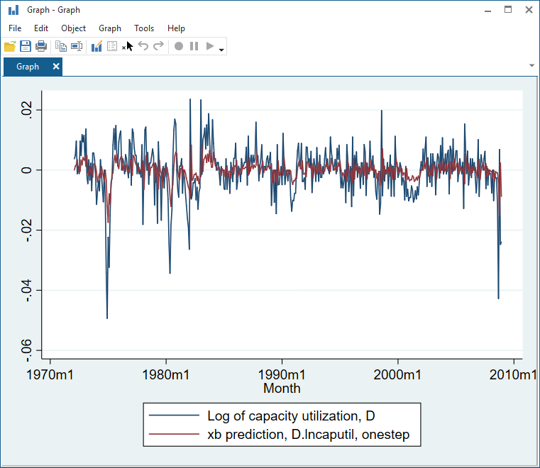
A graph comparing the one-step predictions of the difference in the log of capacity utilization with its predictions is created by typing