In contrast with other econometric software, there is no reason for most users to learn a complicated command language. EViews’ built-in procedures are a mouse-click away and provide the tools most frequently used in practical econometric and forecasting work.

BASIC STATISTICAL ANALYSIS

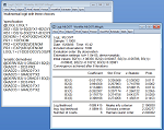
EViews supports a wide range of basic statistical analyses, encompassing everything from simple descriptive statistics to parametric and nonparametric hypothesis tests.

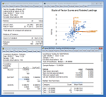
Basic descriptive statistics are quickly and easily computed over an entire sample, by a categorization based on one or more variables, or by cross-section or period in panel or pooled data. Hypothesis tests on mean, median and variance may be carried out, including testing against specific values, testing for equality between series, or testing for equality within a single series when classified by other variables (allowing you to perform one-way ANOVA). Tools for covariance and factor analysis allow you to examine the relationships between variables.

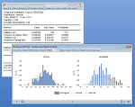
You can visualize the distribution of your data using histograms, theoretical distribution, kernel density, or cumulative distribution, survivor, and quantile plots. QQ-plots (quantile-quantile plots) may be used to compare the distribution of a pair of series, or the distribution of a single series against a variety of theoretical distributions.

You can even perform Kolmogorov-Smirnov, Liliefors, Cramer von Mises, and Anderson-Darling tests to see whether your series is distributed normally, or whether it comes from another distribution such as an exponential, extreme value, logistic, chi-square, Weibull, or gamma distribution.

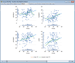
EViews also produces scatter plots with curve fitting using ordinary, transformation, kernel, and nearest neighbor regression.

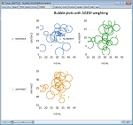
Bubble plots allow you to use a third series to determine the size of the dots in a scatter plot.

Explore the time series properties of your data with tools ranging from simple autocorrelation plots to frequency filters to Q-statistics to unit root tests.

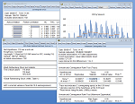
EViews provides autocorrelation and partial autocorrelation functions, Q-statistics, and cross-correlation functions, as well as unit root tests (ADF, Phillips-Perron,  KPSS, DFGLS, ERS, or Ng-Perron for single time series and Levin-Lin-Chu, Breitung, Im-Pesaran-Shin, Fisher, or Hadri for panel data, as well as breakpoint unit root and seasonal unit root tests), cointegration tests (Johansen with MacKinnon-Haug-Michelis critical values and p-values for ordinary data, and Pedroni, Kao, or Fisher for panel data), causality, and independence tests.

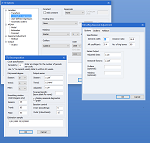
EViews also provides easy-to-use front-end support for the U.S. Census Bureau’s X-13 Seasonal Adjustment programs and MoveReg for weekly data from the U.S. Bureau of Labor Statistics. STL Decomposition provides seasonal adjustment for any frequency data, and simple seasonal adjustment using additive and multiplicative difference methods is also supported in EViews.

You can even use EViews to compute trends and cycles from time series data using the Hodrick-Prescott, Baxter-King, Christiano-Fitzgerald fixed length and Christiano-Fitzgerald asymmetric full sample band-pass (frequency) filters.

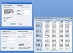
EViews features a wide variety of tools designed to facilitate working with both panel or pooled/time series-cross section data. Define panel structures with virtually no limit on the number of cross-sections or groups, or on the number of periods or observations in a group. Dated or undated, balanced or unbalanced, and regular or irregular frequency panel data sets are all handled naturally within the EViews framework.

Data structure tools facilitate  transforming your data from stacked (panel) to unstacked (pooled) formats, and back again. Smart links, auto series, and data extraction tools, allow you to slice, match merge, frequency convert, and summarize your data with ease.

Support for basic longitudinal data analysis ranges from convenient by-group and by-period statistics, tests, and graphs, to sophisticated panel unit root (Levin-Lin-Chu, Breitung, Im-Pesaran-Shin, or Fisher) and cointegration diagnostics (Pedroni (2004), Pedroni (1999), and Kao, or the Fisher-type test).

Specialized tools for displaying panel data graphs allow you to view stacked, individual, or summary displays. Display line graphs of each graph in a single graph frame or in individual frames. Or show summary statistics for the panel data taken across cross-sections, with mean (or median) and standard deviation (or quantile) bands.

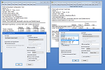
EViews allows you to choose from a full set of basic single equation estimators including: ordinary and nonlinear least squares (multiple regression), weighted least squares, two-stage least squares (instrumental variables), quantile regression (including least absolute deviations estimation), and  stepwise linear regression. Weighted estimation is available for all of  these techniques. Specifications may include polynomial lag structures on any number of independent variables.

For time series analysis, EViews estimates ARMA and ARMAX models, and a wide range of ARCH specifications. Structural time series models may be estimated using the state space object.

In addition to these basic estimators, EViews supports estimation and diagnostics for a variety of advanced models.

Generalized Method of Moments (GMM)

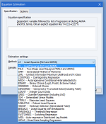
EViews supports GMM estimation for both cross-section and time series data (single and multiple equation). Weighting options include the White covariance matrix for cross-section data and a variety of HAC covariance matrices for time series data. The HAC options include prewhitening, a variety of kernels, and fixed, Andrews, or Newey-West bandwith selection methods. You can estimate a GMM equation using either iterative procedures, or a continuously updating procedure. Post-estimation diagnostics for GMM equations, including weak instrument statistics, are also available.

ARCH

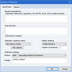
If the variance of your series fluctuates over time, EViews can estimate the path of the variance using a wide variety of Autoregressive Conditional Heteroskedasticity (ARCH) models. EViews handles GARCH(p,q), EGARCH(p,q), TARCH(p,q), PARCH(p,q), and Component GARCH specifications and provides maximum likelihood estimation for errors following a normal, Student’s t or Generalized Error Distribution. The mean equation of ARCH models may include ARCH and ARMA terms, and both the mean and variance equations allow for exogenous variables.

Limited Dependent Variables

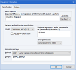
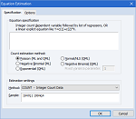
EViews also supports estimation of a range of limited dependent variable models. Binary, ordered, censored, and truncated models may be estimated for likelihood functions based on normal, logistic, and extreme value errors. Count models may use Poisson, negative binomial, and quasi-maximum likelihood (QML) specifications. Heckman Selection models offer two-step or MLE estimation. EViews optionally reports generalized linear model or QML standard errors.

Other Estimatiors

EViews also offers estimation of robust least squares, elastic net, ridge regression, LASSO, functional coefficient, stepwise, MIDAS (mixed frequency) and threshold models.

Panel and Pooled Time Series-Cross Section

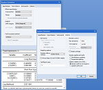
EViews offers various panel and pooled data estimation methods. In addition to ordinary linear and non-linear least-squares, equation estimation methods include 2SLS/IV and Generalized 2SLS/IV, and GMM, which can be used to estimate complex dynamic panel data specifications (including Anderson-Hsiao and Arellano-Bond types of estimators).

Most of the methods allow for both time and cross-section fixed and random effects specifications. For random effects models, quadratic unbiased estimators of component variances include Swamy-Arora, Wallace-Hussain and Wansbeek-Kapteyn.

Also supported are AR specifications (any effects are defined after transformation), weighted least squares, and seemingly unrelated regression. In pools, coefficients for specific variables (including AR terms) can be constrained to be identical, or allowed to differ across  cross-sections.

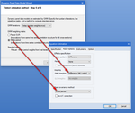
EViews also offers powerful tools for analyzing systems of equations. You may use EViews to estimation of both linear and nonlinear systems of equations by OLS, two-stage least squares, seemingly unrelated regression, three-stage least squares, GMM, and FIML. The system may contain cross equation restrictions and in most cases, autoregressive errors of any order.

Vector Autoregression/Error Correction Models

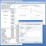
Vector Autoregression, Bayesian VARs, Mixed Frequency VARs, Markov Switching VARs and Vector Error Correction models can be easily estimated by EViews. Once estimated, you may examine the impulse response functions and variance decompositions for the VAR or VEC. VAR impulse response functions and decompositions feature standard errors calculated either analytically or by Monte Carlo methods (analytic not available for decompositions) and may be displayed in a variety of graphical and tabular formats.

You may impose and test linear restrictions on the cointegrating relations and/or adjustment coefficients. EViews’ VARs also allow you to estimate structural factorizations (VARs) by imposing short-run (Sims 1986) or long-run (Blanchard and Quah 1989) restrictions, or both. Over-identifying restrictions may be tested using the LR statistic reported by EViews.

VARs support a variety of views to allow you to examine the structure of your estimated specification. With a few clicks of the mouse, you can display the inverse roots of the characteristic AR polynomial, perform Granger causality and joint lag exclusion tests, evaluate various lag length criteria, view correlograms and autocorrelations, or perform various multivariate residual based diagnostics.

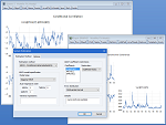
Multivariate ARCHMultivariate ARCH is useful in modeling time varying variance and covariance of multiple time series. A number of popular ARCH models, such as the Conditional Constant Correlation (CCC), the Diagonal VECH, and the Diagonal BEKK, are available. Exogenous variables are allowed in the mean and variance equations; nonlinear and AR terms can be included in the mean equations. The error is assumed to distributed either as multivariate Normal or Student’s t. Bollerslev-Wooldridge robust standard errors are also available. Once the model is estimated, users can easily generate the in-sample variance, covariance, or correlation, in tabular or graphic format.

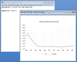
State-Space ModelsThe state-space object allows estimation of a wide variety of single- and multi-equation dynamic time-series models using the Kalman Filter algorithm. Among other things, you can use the state-space object to estimate random and time-varying coefficient models and ML ARMA specifications.

Sophisticated procs and views give you access to powerful filtering and smoothing tools so that you can view or generate one-step ahead, filtered, or smoothed signals, states, or errors. EViews’ built-in forecasting procedures also provide easy-to-use tools for in- and out-of-sample forecasting using n-step ahead or smoothed values.

For custom analysis, EViews’ easy-to-use likelihood object permits estimation of user-specified maximum likelihood models. You simply provide standard EViews expressions to describe the log likelihood contributions for each observation in your sample, set coefficient starting values, and EViews will do the rest.