MULTILEVEL META-ANALYSIS IN ACTION!

EXAMPLE DATASET: MODIFIED SCHOOL CALENDAR DATA

Many studies suggest that the long summer break at the end of a school year is linked to a learning gap between students because of students’ differential access to learning opportunities in the summer.

 

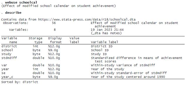
Cooper, Valentine, and Melson (2003) conducted a multilevel meta-analysis on schools that modified their calendars without prolonging the school year. The dataset consists of 56 studies that were conducted in 11 school districts. Some schools adopted modified calendars that featured shorter breaks more frequently throughout the year (for example, 12 weeks of school followed by 4 weeks off) as opposed to the traditional calendar with a longer summer break and shorter winter and spring breaks. The studies compared the academic achievement of students on a traditional calendar with those on a modified calendar. The effect size (stdmdiff) is the standardized mean difference, with positive values indicating higher achievement, on average, in the group on the modified calendar. The standard error (se) of stdmdiff was also reported by each study. Let’s first describe our dataset:

 

MULTILEVEL META-ANALYSIS: CONSTANT-ONLY MODEL

Because the schools are nested within districts, we fit a three-level random-intercepts model. This requires that we specify two random-effects equations: one for level 3 (identified by variable district) and one for level 2 (identified by variable school).

 

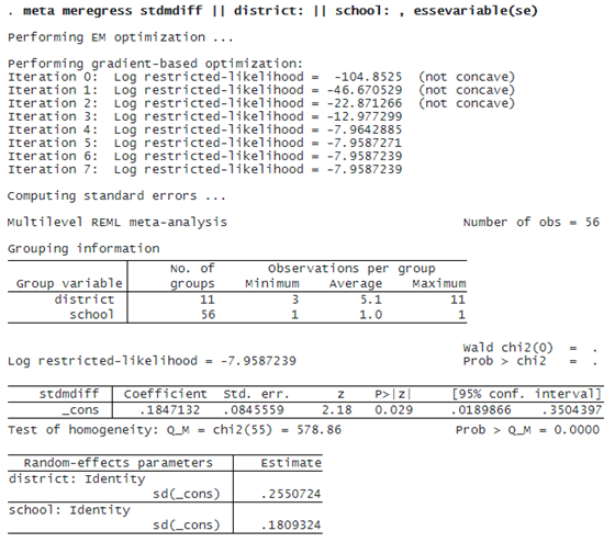
The first table displays information on groups at different levels of hierarchy with one row for each grouping (level of hierarchy).

 

The second table displays the fixed-effects coefficients. Here there is only an intercept corresponding to the overall effect size θ^. The value of θ is 0.185 with a 95% CI of [0.019, 0.35]. This means that, on average, students following the modified school calendar achieved higher scores than those who did not.

 

The third table displays the random-effects parameters, traditionally known as variance components in the context of multilevel or mixed-effects models. The variance-component estimates are now organized and labeled according to each level. By default, meta meregress reports standard deviations of the random intercepts (and correlations if they existed in the model) at each level. But you can instead specify the variance option to report variances (and covariances if they existed in the model). We have τ3^=0.255 and τ2^=0.181. These values are the building blocks for assessing heterogeneity across different hierarchical levels and are typically interpreted in that context. In general, the higher the value of τl, the more heterogeneity is expected among the groups within level l.

 

Alternatively, this can be specified using the meta multilevel command as follows:

 

. meta multilevel stdmdiff, relevels(district school) essevariable(se)
(output omitted)

 

The meta multilevel command was designed to fit random-intercepts meta-regression models, which are commonly used in practice. It is a convenience wrapper for meta meregress.

 

MULTILEVEL HETEROGENEITY

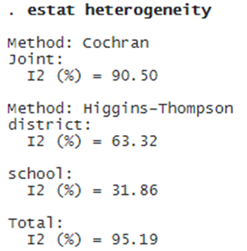
We will use the postestimation command estat heterogeneity to quantify the multilevel heterogeneity among the effect sizes.

 

 

© Copyright 1996–2024 StataCorp LLC. All rights reserved.

Cochran’s I2 quantifies the amount of heterogeneity jointly for all levels of hierarchy. I2=90.50% means that 90.50% of the variability among the effect sizes is due to true heterogeneity in our data as opposed to the sampling variability.

 

The multilevel Higgins–Thompson I2 statistics assess the contribution of each level of hierarchy to the total heterogeneity, in addition to their joint contribution. For example, between-schools heterogeneity or heterogeneity within districts (level 2 heterogeneity) is the lowest, accounting for about 32% of the total variation in our data, whereas between-districts heterogeneity (level 3 heterogeneity) accounts for about 63% of the total variation.

 

MULTILEVEL META-REGRESSION AND RANDOM SLOPES: INCORPORATING MODERATORS

We will use variable year_c to conduct a three-level meta-regression and include random slopes (corresponding to variable year_c) at the district level.

 

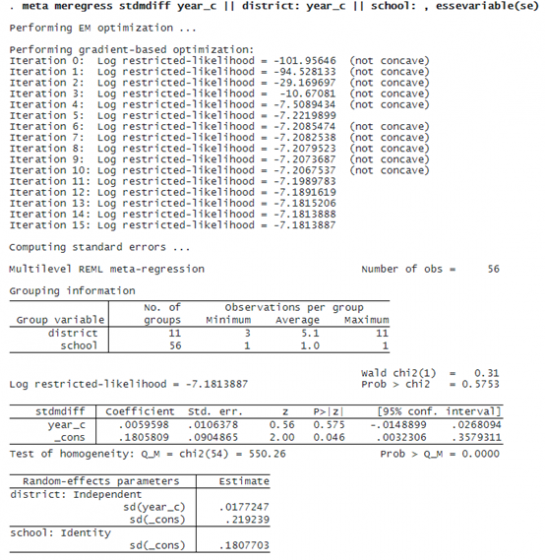
The estimate of the regression coefficient of variable year_c is 0.006 with a 95% CI of [–0.015, 0.027] . We do not see any evidence for the association between stdmdiff and year_c (p = 0.575).

 

RANDOM-EFFECTS COVARIANCE STRUCTURES

Although year_c did not explain the heterogeneity, we continue to include it as a moderator for illustration purposes.

 

By default, the random slopes and random intercepts (at the district level) are assumed independent. Alternatively, we can specify an exchangeable covariance structure using option covariance(exchangeable). We suppress the header and the iteration log and display results with three decimal points using the noheader, nolog, and cformat(%9.3f) options.

 

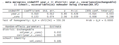
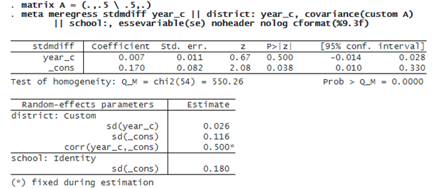
Alternatively, we can specify a custom covariance structure by fixing the correlation between the intercepts and slopes at 0.5 and allowing for their standard deviations to be estimated from the data:

 

 

PREDICTING RANDOM EFFECTS

Below, we predict the random effects using predict, reffects and obtain their diagnostic standard errors by specifying the reses(, diagnostic) option.

 

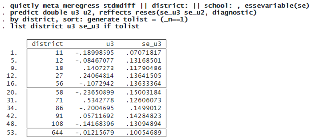
The random intercepts u3 are district-specific deviations from the overall mean effect size. For example, for district 18, the predicted standardized mean difference is 0.14 higher than the overall effect size.