META-ANALYSIS FOR PREVALENCE IN ACTION!

EXAMPLE DATASET: PROPORTIONS OF VEGETARIANS ACROSS THE SEVEN REGIONS OF THE U.S.

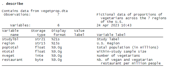
Meeting your future in-laws for the first time can be nerve-racking. You decided to impress your future mother-in-law, who plans on opening an online restaurant that delivers food across the United States. Being the statistician in the family, you suggested conducting an MA to assess the overall proportion of vegetarians (and vegans) across the seven regions of the U.S. Guided by the results of the MA, you hope to help the restaurant tailor more vegetarian-friendly recipes to specific regions of the U.S. For simplicity, assume you identified one study in each region to include in the MA.

 

META-ANALYSIS OF ONE-SAMPLE BINARY DATA

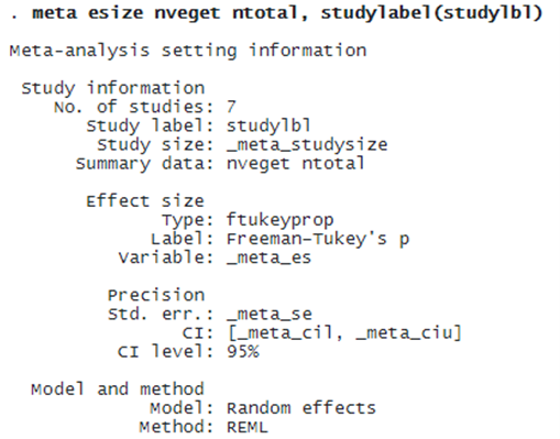
Variables nveget and ntotal represent the number of vegetarians and the total number of subjects in each study. By default, meta esize computes the Freeman–Tukey double-arcsine-transformed proportion for each study. This is a variance-stabilizing transformation and is particularly preferable when the proportions are close to 0 or 1.

 

DECLARE YOUR DATA AS META DATA VIA META ESIZE

 

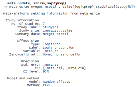
You may specify the logit-transformed proportion as the effect size using option esize(logitprop). Because the variance of the logit-transformed proportion depends on the proportion itself, the MA of this effect size tends to assign artificially low weights for studies with proportions close to 0 or 1.

 

Perhaps you may wish to compute the untransformed proportions; however, this is recommended only if all the proportions reported by the studies are close to .5, which is not common in practice.

 

© Copyright 1996–2024 StataCorp LLC. All rights reserved.

 

. meta update, esize(proportion)
(Output omitted)

 

FOREST PLOTS AND OTHER META-ANALYSIS TECHNIQUES

Continuing with the first specification of meta esize, after computing the effect size of interest and declaring your data as meta data, you may use any MA technique as usual. For example, to construct a forest plot, we type

 

. meta forest, proportion

The proportion option specifies that the results be reported as proportions instead of the default Freeman–Tukey-transformed proportions. This is equivalent to applying the inverse Freeman–Tukey transformation using option transform(invftukey). The overall (mean) proportion of vegetarians is .06 with a CI of [.04, .08].

 

You may also report your results as, say, the number of vegetarians per 1,000 persons using suboption scale() of option transform(). We will also show the corresponding region (variable region) of each study on the forest plot.

 

. meta forest _id _data region _plot _esci _weight,
  transform(invftukey, scale(1000)) esrefline insidemarker

The above forest plots revealed substantive differences among the proportions of vegetarians, with higher prevalence of vegetarians in the Pacific Coastal, New England, and Mid-Atlantic regions compared with the rest of the U.S. regions.

 

The meeting with the in-laws is around the corner. Luckily for you, backed with the above forest plot, you may advise your future mother-in-law to incorporate more vegetarian recipes on her menu for the aforementioned regions and color her impressed!