Model selection is fundamental to any statistical analysis, and information criteria have been and remain some of the more common statistical techniques for model selection. In Stata, after any estimation command that reports a log likelihoood, which includes most estimation commands, simply type
. estat ic, aiccorrected
or
. estat ic, aicconsistent
to compute AICc or CAIC, respectively.
To report all four information criteria (AIC, BIC, AICc, and CAIC), type
. estat ic, all
Sometimes, in analyses such as linear mixed models, we need to manually specify the degrees of freedom or the number of observations to be used in the calculation of the criterion. We can do this by specifying options n() and df():
. estat ic, n(500) df(10) all
These same new criteria and options are also available with the estimates stats command.
CORRECTED AIC AND CONSISTENT AIC IN ACTION!
USING INFORMATION CRITERIA FOR A SMALL SAMPLE SIZE
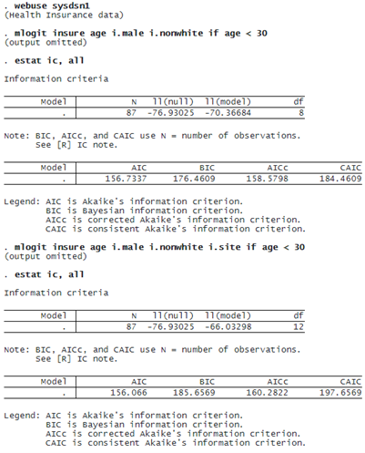
We start by exploring information criteria for a dataset with a small sample size. In such datasets, AICc is considered a more reliable criterion than AIC. We compare two multinomial models for insurance type without and with the site dummy variable. The dummy variable site indicates the site of study. We also include the age<30 condition to reduce the sample size to only 87 observations.

© Copyright 1996–2025 StataCorp LLC. All rights reserved.
The AIC suggests that the model with the site dummies is preferred, whereas the AICc suggests the opposite.
SPECIFYING DEGREES OF FREEDOM
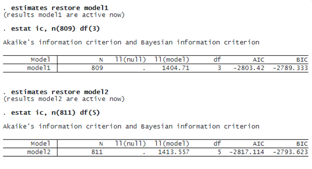
As we mentioned earlier, when fitting linear mixed models using restricted maximum likelihood, care must be taken when comparing models, especially when the fixed-effects specification differs across models. We show how to use the n() and df() options to modify the default values of the number of observations and degrees of freedom that are used for the computation of information criteria. Suppose we want to compare the following two models:
. webuse productivity
(Public capital productivity)

. mixed gsp private emp hwy water other unemp || region: || state:, reml
(output omitted)

. estimates store model1

. mixed gsp private emp hwy unemp || region: hwy || state: unemp, reml
(output omitted)

. estimates store model2
The two models differ in both their fixed-effects and random-effects specifications. Therefore, it is not reliable to compare models with the standard information criteria. Below, we manually specify n() and df() to make models comparable. For each model, the value of n() is computed by subtracting the number of fixed-effects parameters from the number of observations, and df() indicates the number of random-effects parameters.

Both AIC and BIC indicate that the second model is preferable.

