INDIVIDUALIZED AVERAGE TREATMENT EFFECTS
We want to estimate the effect of 401(k) eligibility (e401k) on net financial assets (asset) to answer the following questions:
- Are the effects of 401(k) eligibility on net wealth heterogeneous? In other words, do the treatment effects vary across individuals or groups?
- If the treatment effects are heterogeneous, how do the treatment effects vary across prespecified groups, such as income categories?
The data are from a sample of households in the 1990 Survey of Income and Program Participation (SIPP). They contain information on the head of the household: income level category (incomecat), age (age), years of education (educ), whether they receive a pension benefit (pension), marital status (married), whether they participate in an IRA (ira), whether they own a home (ownhome), and whether there are two earners in the same household (twoearn).
We want to study the effect of being eligible for a 401(k) on assets (assets) given a person’s incomecat, age, educ, pension, married, ira, ownhome, and twoearn. With teffects, for instance, we can get an average effect. With cate, we can get an effect for each individual, an individualized average treatment effect (IATE).
First, we open the assets3 dataset. To save some typing later, we define a global macro, catecovars, that stores the names of the variables on which we will condition.
. use https://www.stata-press.com/data/r18/assets3
(Excerpt from Chernozhukov and Hansen (2004))

. global catecovars age educ i.(incomecat pension married twoearn ira ownhome)
We are ready to fit the model using cate. We specify po following the command name to use the partialing-out estimator. We specify the outcome variable asset and the global macro $catecovars that contains the predictors in the first set of parentheses and the treatment-assignment variable e401k in the second set of parentheses. We also specify the rseed() option to make the results reproducible.
. cate po (assets $catecovars) (e401k), rseed(12345671)

Cross-fit fold 1 of 10 ...
Performing lasso for outcome assets ...
Performing lasso for treatment e401k ...

Cross-fit fold 2 of 10 ...
Performing lasso for outcome assets ...
Performing lasso for treatment e401k ...

Cross-fit fold 3 of 10 ...
Performing lasso for outcome assets ...
Performing lasso for treatment e401k ...

Cross-fit fold 4 of 10 ...
Performing lasso for outcome assets ...
Performing lasso for treatment e401k ...

Cross-fit fold 5 of 10 ...
Performing lasso for outcome assets ...
Performing lasso for treatment e401k ...

Cross-fit fold 6 of 10 ...
Performing lasso for outcome assets ...
Performing lasso for treatment e401k ...

Cross-fit fold 7 of 10 ...
Performing lasso for outcome assets ...
Performing lasso for treatment e401k ...

Cross-fit fold 8 of 10 ...
Performing lasso for outcome assets ...
Performing lasso for treatment e401k ...

Cross-fit fold 9 of 10 ...
Performing lasso for outcome assets ...
Performing lasso for treatment e401k ...

Cross-fit fold 10 of 10 ...
Performing lasso for outcome assets ...
Performing lasso for treatment e401k ...

Performing random forest for IATE ...
Estimating AIPW scores ...
Estimating ATE ...

Conditional average treatment effects     Number of observations       = 9,913
Estimator:       Partialing out           Number of folds in cross-fit =    10
Outcome model:   Linear lasso             Number of outcome controls   =    17
Treatment model: Logit lasso              Number of treatment controls =    17
CATE model:      Random forest            Number of CATE variables     =    17
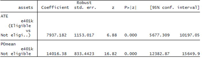
The iteration log shows the cross-fitting process of fitting the outcome model to assets and the treatment model to e401k. By default, lasso for the linear model is used for the outcome assets, and lasso for the logit model is used for the treatment e401k.
The output shows that random forest is used to estimate the IATE function once the cross-fitting is finished. Then the AIPW scores implied by the partial linear model are computed, and the ATE is estimated as an average of the AIPW scores. The ATE reported in the table indicates that if everyone in the population were eligible for a 401(k), the net financial assets would be, on average, $7,937 higher than if no one were eligible for 401(k).
In addition to the ATE, cate estimates IATEs, which we can use to predict treatment effects for each observation. First, we use categraph histogram to draw a histogram of the predicted IATEs and see their distribution.
. categraph histogram

The graph shows that treatment effects are mostly positive but have a fat right tail. Thus, the ATE may underestimate the effect of 401(k) eligibility on assets for some groups.
Although the histogram above allows us to visually inspect the distribution of treatment effects, we should not use it as evidence to support treatment-effects heterogeneity. To test whether the treatment effects are heterogeneous, use estat heterogeneity.
. estat heterogeneity

Treatment-effects heterogeneity test
H0: Treatment effects are homogeneous

    chi2(1) =   4.11
Prob > chi2 = 0.0427
© Copyright 1996–2025 StataCorp LLC. All rights reserved.
We can further explore heterogeneity. We might want to see how the IATE function changes across levels of a variable of interest while fixing all other covariates at specified values, such as their means. For example, we can allow educ to vary while holding the other variables fixed.
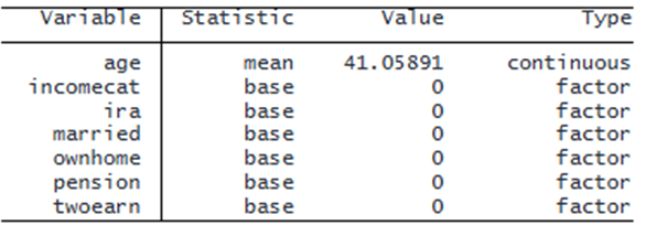
We use categraph iateplot to visually examine the change in the IATE function across educ levels. By default, the continuous variables such as age are fixed at their sample means, and the factor variables are fixed at their base levels.
. categraph iateplot educ

Note: IATE estimated at fixed values of covariates other than educ.

In addition to the IATE function, categraph iateplot plots the 95% pointwise confidence intervals for the predictions. Below 10 years of education, the effects seem constant. The graph shows that the treatment effects are larger for people with 12 to 15 years of education while holding other variables fixed. After 15 years of education, there is more variability, and the confidence intervals are wider, making it difficult to determine whether the effect changes at these high education levels.
ESTIMATING TREATMENT EFFECTS OVER PRESPECIFIED GROUPS
Above, we learned that the treatment effects of 401(k) eligibility on financial assets are heterogeneous. To characterize the heterogeneous effects, we want to know how the average treatment effects vary across prespecified groups, such as income categories.
We first look at the minimum, maximum, and median income in each income category.
. table incomecat, stat(min income) stat(max income)
     stat(median income) nototal
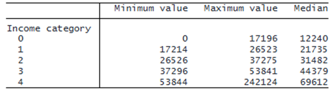
We see that levels 0 and 1 refer to low-income groups, levels 2 and 3 refer to middle-level income groups, and level 4 refers to high- income groups.
We have already estimated the IATE function; we now estimate group average treatment effects (GATEs), which are summaries of the IATE function for each level of a group variable. Thus, there is no need to reestimate the IATE function; we can use the existing IATE function. With cate, we specify the reestimate option to reestimate effects without reestimating the IATE function. This option will save computation time. We specify the group(incomecat) option to estimate GATEs for the income categories.
. cate, group(incomecat) reestimate

Estimating GATE ...

Conditional average treatment effects     Number of observations       = 9,913
Estimator:       Partialing out           Number of folds in cross-fit =    10
Outcome model:   Linear lasso             Number of outcome controls   =    17
Treatment model: Logit lasso              Number of treatment controls =    17
CATE model:      Random forest            Number of CATE variables     =    17
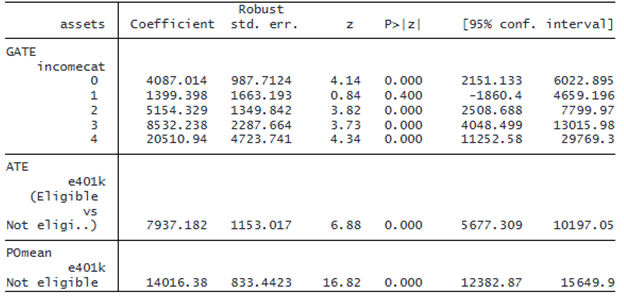
The results show both ATE and GATEs. For example, the GATE for the high-income group (level 4) is $20,511. For the highest income group, being eligible for 401(k) is expected to increase their net financial assets by $20,511 compared with the net financial assets if not eligible for 401(k). In contrast, the GATE estimate for the lowest income group (level 0) is only $4,087. In other words, people who earn more benefit more from working in a company with a 401(k) plan. The ATE estimate indicates that treatment effects for the population are expected to be $7,937. Thus, using the ATE alone does not fully characterize treatment effects among different income categories.
We can use categraph gateplot to visualize the GATE estimates to see if there is any trend.
. categraph gateplot

The graph confirms an upward trend. To further test if there is treatment-effects heterogeneity among the income groups, we use estat gatetest.
. estat gatetest

Group treatment-effects heterogeneity test
H0: Group average treatment effects are homogeneous

 ( 1)  [GATE]0bn.incomecat - [GATE]1.incomecat = 0
 ( 2)  [GATE]0bn.incomecat - [GATE]2.incomecat = 0
 ( 3)  [GATE]0bn.incomecat - [GATE]3.incomecat = 0
 ( 4)  [GATE]0bn.incomecat - [GATE]4.incomecat = 0

    chi2(4) =  18.44
Prob > chi2 = 0.0010
The test formally confirms what we see on the graph. We have strong evidence to suggest that the effects are not homogeneous.