Consider the diabetes dataset, which contains records of disease progression in 442 patients along with control factors such as age, gender, body mass index, blood pressure, and measurements on their blood serum (Efron et al. 2004).
. webuse diabetes
(2004 Diabetes progression data)
Following a common procedure in variable-selection methodologies, all variables are standardized so that they have mean 0 and standard deviation of 1. The outcome variable of interest is diabetes, which we regress on the other 10 variables. We assume that not all covariates are of equal importance and that by performing variable selection, we can achieve more efficient inference and improved prediction.
Performing Bayesian variable selection with bayesselect is as simple as any other regression in Stata. We use the default specification of bayesselect, and the only option we add is rseed() for reproducibility. When fitting the model, we exclude the last observation, the 442th, to be used as a test case later.
. bayesselect diabetes age sex bmi bp serum1-serum6 in 1/441, rseed(19)

Burn-in ...
Simulation ...

Model summary
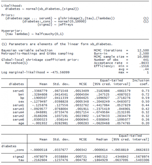
The default variable selection prior used by bayesselect is the horseshoe prior (Carvalho, Polson, and Scott 2009). It is a special case of the so-called global–local shrinkage priors that include local shrinkage factors lambdas, one for each coefficient. The form of this prior is described in the model summary of the command.
The shrinkage factors are transformed into inclusion coefficients and summarized in the last column of the output of bayesselect. The predictor variables in the output are ordered by inclusion coefficients. The top three predictors, which have inclusion coefficients greater than 0.5, are serum5, bmi (body mass index), and bp (blood pressure). All three of these predictors have positive effects on the outcome—the posterior mean estimates for their coefficients are 0.34, 0.33, and 0.19, respectively.
In a second output table, below the table with coefficients, bayesselect reports posterior summaries for the constant term, the variance term sigma2, and the global shrinkage parameter tau.
Because we want predictions, we first need to save the simulation results from bayesselect.
. bayesselect, saving(model1sim)
note: file model1sim.dta saved.
We can now use the bayespredict command to predict disease progression for the last patient in the study, observation 442.
© Copyright 1996–2025 StataCorp LLC. All rights reserved.
. bayespredict double pmean1 in 442, mean
The computed posterior predictive mean is saved in a new variable, pmean1. We will look at this prediction later.
Another popular variable-selection model is the spike-and-slab lasso model (Ročková and George 2018). We request this model by specifying the sslaplace option with bayesselect.
. bayesselect diabetes age sex bmi bp serum1-serum6 in 1/441, sslaplace rseed(19)

Burn-in ...
Simulation ...

Model summary
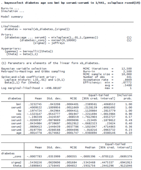
Instead of the inclusion coefficients of the horseshoe prior model, the output of spike-and-slab lasso reports inclusion probabilities, which are easier to interpret. The predictors serum5, bmi, and bp all have perfect inclusion, 1. In other words, there is no uncertainty about the importance of these three predictors. Their coefficient estimates, however, are similar to those of the horseshoe prior model.
Let’s save the last simulation results and make a prediction for the last patient in the study.
. bayesselect, saving(model2sim)
note: file model2sim.dta saved.

. bayespredict double pmean2 in 442, mean
To compare the prediction results of the two variable-selection models, we list the record of observation 442.
. list in 442
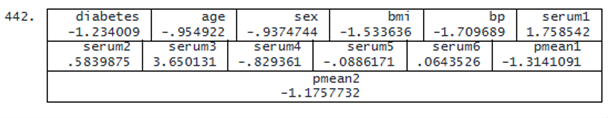
The prediction of the spike-and-slab model (−1.18) is closer to the true value (−1.23) than the prediction of the horseshoe prior model (−1.31). In conclusion, both models correctly predict slowing of disease progression for this patient.