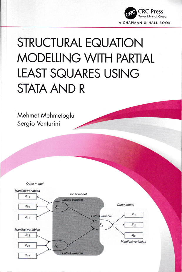
Structural equation modeling (SEM) is a statistical framework that can model both observed and unobserved (latent) variables through complex relationships. While the traditional covariance-based SEM aims to find parameter estimates that minimize the distance between the observed and model-implied covariances of the observed variables, partial least-squares SEM (PLS-SEM) aims to find parameter estimates that maximize explained variance.
Structural Equation Modelling with Partial Least Squares Using Stata and R, by Mehmet Mehmetoglu and Sergio Venturini, offers a comprehensive tutorial on conducting PLS-SEM and consistent PLS-SEM through the author’s open-source plssem package.
The authors begin with theoretical introductions to PLS-SEM and various multivariate statistical prerequisites. The following chapters provide a step-by-step guide to conducting PLS-SEM in Stata, including model specification, estimation, assessment, and interpretation. The remaining chapters introduce concepts and examples for mediation, moderation, and detecting unobserved heterogeneity in PLS-SEM and close with some advice and an example of writing up a PLS-SEM study. The datasets and do-files from all the examples are available as a GitHub repository at https://github.com/sergioventurini/SEMwPLS.
Structural Equation Modelling with Partial Least Squares Using Stata and R is a useful resource for researchers interested in learning more about PLS-SEM and for more advanced researchers interested in learning how to fit PLS-SEM models in Stata.
1.2 Two Approaches to Estimating SEM Models
1.2.2 Partial least squares SEM
1.2.3 Consistent partial least squares SEM
1.3 What Analyses Can PLS-SEM Do?
1.4 The Language of PLS-SEM
1.5 Summary
2.2 Principal Component Analysis
2.3 Segmentation Methods
2.3.1 Cluster analysis
2.3.1.2 Partitional clustering algorthms
2.3.2 Finite mixture models and model-based clustering
2.3.3 Latent class analysis
2.4 Path Analysis
2.5 Getting to Partial Least Squares Structural Equation Modelling
2.6 Summary
Appendix: R Commands
Principal component analysis
Segmentation methods
Latent class analysis
Path analysis
Appendix: Technical Details
The algebra of principal components analysis
Clustering stopping rules
Finite mixture models estimation and selection
Path analysis using matrices
3.2 Model specification
3.2.2 Inner (structural) model
3.2.3 Application: Tourists satisfaction
3.3 Model Estimation
3.3.2 Stage I: Iterative estimation of latent variable scores
3.3.3 Stage II: Estimation of measurement model parameters
3.3.4 Stage III: Estimation of structural model parameters
3.4 Bootstrap-based Inference
3.5 The plssem Stata Package
3.5.2 Options
3.5.3 Stored results
3.5.4 Application: Tourists satisfaction (cont.)
3.6 Missing Data
3.7 Effect Decomposition
3.8 Sample Size Requirement
3.9 Consistent PLS-SEM
3.10 Higher Order Constructs
3.11 Summary
Appendix: R Commands
The cSEM package
Appendix: Technical Details
More details on the consistent PLS-SEM approach
4.2 Assessing the Measurement Part
4.2.1 Reflective measurement models
4.2.1.2 Construct reliability
4.2.1.3 Construct validity
4.2.2 Higher order reflective measurement models
4.2.3 Formative measurement models
4.2.3.2 Multicollinearity
4.2.3.3 Weights
4.3 Assessing the Structural Part
4.3.2 Goodness-of-fit
4.3.3 Path coefficients
4.4 Assessing a PLS-SEM Model: A Full Example
4.4.2 Estimation using plssem in Stata
4.4.3 Evaluation of the example study model
4.4.3.2 Structural part
4.5 Summary
Appendix: R Commands
Appendix: Technical Details
Tools for assessing the structural part of a PLS-SEM model
5.2 Baron and Kenny’s Approach to Mediation Analysis
5.2.2 Alternative to the Baron-Kenny approach
5.2.3 Effect size of the mediation
5.3 Examples in Stata
5.3.2 Example 2: A single latent mediator variable
5.3.3 Example 3: Multiiple latent mediator variables
5.4 Moderated Mediation
5.5 Summary
Appendix: R Commands
6.2 Product-Indicator Approach
6.3 Two-Stage Approach
6.4 Multi-Sample Approach
6.4.2 Permutation test
6.5 Example Study: Interaction Effects
6.5.2 Application of the two-stage approach
6.5.2.2 Two-stage with a categorical moderator
6.5.3 Application of the multi-sample approach
6.6 Measurement Model Invariance
6.7 Summary
Appendix: R Commands
Application of the two-stage approach
Application of the multi-sample approach
Measurement model invariance
7.2 Methods for the Identification and Estimation of Unobserved Heterogeneity in PLS-SEM
7.2.2 Finite mixture PLS (FIMIX-PLS)
7.2.3 Other methods
7.2.3.2 Partial least squares genetic algorithm segmentation (PLS-GAS)
7.3 Summary
Appendix: R Commands
Appendix: Technical Details
Permutation tests
8.2 Example of PLS-SEM Publication
8.3 Summary
A.2 Linear Regression Analysis
A.2.2 Goodness-of-fit
A.2.3 The multiple linear regression model
A.2.4 Inference for the linear regression model
A.2.5 Categorical predictors
A.2.6 Multicollinearity
A.2.7 Example
A.3 Summary
Appendix: R Commands


