We study the effect on wages of time-varying variables, such as age or tenure. At the same time, we are interested in the effects of time-invariant variables, such as race. An FE model will omit any variable that remains constant across time and thus cannot fully answer our research question. An RE model may yield inconsistent estimates because of the possible correlation between individual time-invariant heterogeneity and the regressors age and tenure.
We can use a CRE model to circumvent both problems. Let’s see it in action.
. webuse nlswork
(National Longitudinal Survey of Young Women, 14-24 years old in 1968)
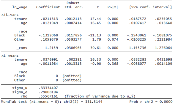
. xtreg ln_wage tenure age i.race, cre vce(cluster idcode)
note: 2.race omitted from xt_means because of collinearity.
note: 3.race omitted from xt_means because of collinearity.
Correlated random-effects regression Number of obs = 28,101
Group variable: idcode Number of groups = 4,699
R-squared: Obs per group:
Within = 0.1296 min = 1
Between = 0.2346 avg = 6.0
Overall = 0.1890 max = 15
Wald chi2(4) = 1685.18
corr(xit_vars*b, xt_means*γ) = 0.5474 Prob > chi2 = 0.0000
(Std. err. adjusted for 4,699 clusters in idcode)
© Copyright 1996–2025 StataCorp LLC. All rights reserved.
Mundlak test (xt_means = 0): chi2(2) = 331.5144 Prob > chi2 = 0.0000
xtreg, cre reports coefficients for the variables in the model (xit_vars) and for their respective panel means (xt_means). In CRE models, panel means are added to the regression to control for potential endogeneity and to correct bias. This procedure gives us the same coefficients we obtain from the corresponding FE model for the time-varying regressors:
. xtreg ln_wage tenure age, fe vce(cluster idcode)

Fixed-effects (within) regression               Number of obs     =     28,101
Group variable: idcode                          Number of groups  =      4,699

R-squared:                                      Obs per group:
     Within  = 0.1296                                         min =          1
     Between = 0.1916                                         avg =        6.0
     Overall = 0.1456                                         max =         15

                                                F(2, 4698)        =     766.79
corr(u_i, Xb) = 0.1302                          Prob > F          =     0.0000

                             (Std. err. adjusted for 4,699 clusters in idcode)
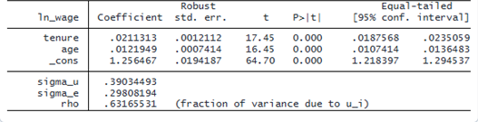
We get the benefits of an FE model but do not lose information about time-invariant features of our model.
xtreg, cre performs a Mundlak specification test to help you choose between an RE and FE or CRE model. Unlike a Hausman test, this test is fully robust and remains valid even when a robust vce(), such as vce(cluster idcode), is specified. From the earlier output of xtreg, cre, the Mundlak test, reported beneath the coefficient table, provides strong evidence in favor of the CRE model.