We have data first analyzed by Dahlberg and Johansson (2000) on expenditures, revenues, and government grants for 265 municipalities in Sweden. We want to see how they alter their spending and taxing behavior in response to grants from the central government. We have nine years of annual data for each municipality. Nine observations would be insufficient to fit a time-series VAR model, but because we have observations for a panel of different municipalities, we can perform a panel-data VAR analysis.
Let’s load the data and fit a model. We specify the lags(2) option with the xtvar command to include two lags of each dependent variable in each equation:
. webuse swedishgov.dta
(1979-1987 Swedish municipality data)
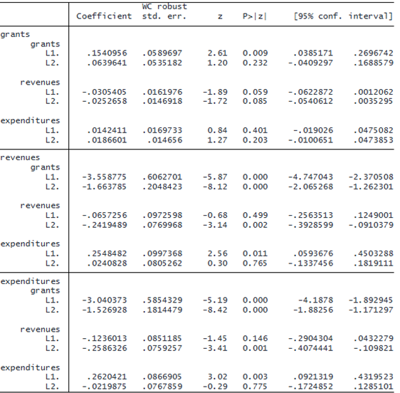
. xtvar grants revenues expenditures, lags(2)
Panel-data vector autoregression Number of obs = 1,590
Group variable: idcode Number of groups = 265
Time variable: year Obs per group:
min = 6
Number of moment conditions = 243 avg = 6.0
max = 6
Fixed-effects transform: FOD
Two-step results
(Std. err. adjusted for 265 clusters in idcode)
Hansen's test of overid. restrictions: chi2(225) = 261.92   Prob > chi2 = 0.046
GMM-type instruments: L(2/.).(grants revenues expenditures)
© Copyright 1996–2025 StataCorp LLC. All rights reserved.
Interpreting the raw coefficients from a panel-data VAR model is not terribly illuminating, but xtvar‘s postestimation commands make obtaining insights easy. We first perform a Granger causality test to see whether grants Granger-causes expenditures. Granger causality is a rather weak notion of causality; it simply asks whether lagged values of one variable are useful in predicting another variable. To do this, we can use the same vargranger command that works after fitting time-series VAR models:
. vargranger

Granger causality Wald tests
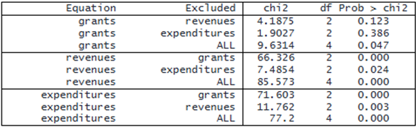
Looking at the equation for expenditures, we see that grants does Granger-cause expenditures. The χ2χ2 statistic is 71.6 with 2 degrees of freedom, which provides evidence to reject the null hypothesis of no Granger causality. In other words, if we were to forecast expenditures, we would obtain a lower mean squared prediction error if we included lags of grants in addition to lags of expenditures and lags of revenues.
We can also use the irf suite of commands to obtain IRFs after fitting a panel-data VAR model. We first use irf create to compute IRFs based on the results of our model. We then use the irf graph command to graph the IRFs and evaluate how a shock to each variable is expected to affect the trajectories of each variable in the next eight time periods.
. irf create baseline, set(swedish_govt_irfs)
(file swedish_govt_irfs.irf created)
(file swedish_govt_irfs.irf now active)
(file swedish_govt_irfs.irf updated)

. irf graph irf, byopt(yrescale)

Looking at the plot in the first column of the second row, we see our simple IRF indicates that an unanticipated grant to a municipality leads to lower expenditures in the two years after the grant is received but then returns to the initial spending level.
xtvar also has postestimation tools that allow us to explore the robustness of our findings; these tools are similar to those you would use after fitting a VAR model. For instance, we could investigate the choice of lag length and instruments used to identify the parameters and find an alternative specification using xtvarsoc. And you can check for stability using varstable.