Let’s explore the relationship between household income and food expenditure using the data from Engel (1857), which are described in Koenker and Bassett (1982). Let’s use a quantile regression to compare this relationship across different quantiles. We first fit a model to the 50th percentile of the outcome variable, a model known as median regression, using default settings. We specify the rseed(19) option for reproducibility.
. webuse engel1857
(European household budget survey)

. bayes, rseed(19): qreg foodexp income

Burn-in ...
Simulation ...

Model summary
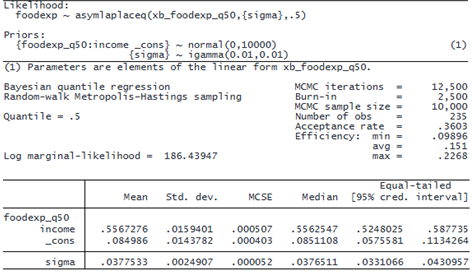
The mean posterior estimate for the coefficient of income is 0.56 with a 95% credible interval (CrI) of [0.52, 0.59]. We now shift our attention to the 25th percentile (or 0.25 quantile) of the outcome variable by specifying the quantile() option with qreg.
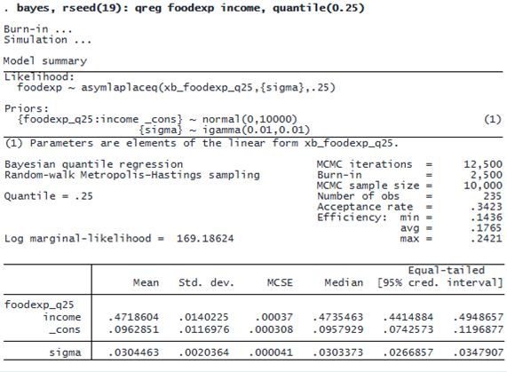
. bayes, rseed(19): qreg foodexp income, quantile(0.25)

Burn-in ...
Simulation ...

Model summary
© Copyright 1996–2025 StataCorp LLC. All rights reserved.
The mean posterior estimate for the coefficient of income is 0.47 with a 95% CrI of [0.44, 0.49]. The CrIs from the two quantile regressions are not overlapping, which suggests that the relationship between income and food expenditure is different between the 0.25 and 0.50 quantiles. We can explore this relationship further by specifying different quantiles in the quantile() option with bayes: qreg and using the results to produce the graph below:

The graph demonstrates heterogeneity of the income coefficients across the distribution (quantiles) of food expenditure. The coefficient increases as the quantile value increases. (This does not mean that the proportion of income spent on food increases with income. If we were to obtain predictions and produce the Engel curve, we would see that food expenditure share decreases with income, as expected.)
All existing Bayesian postestimation commands are available after bayes: qreg. For example, we can compute the posterior probability for the income coefficient in the model for the 25th percentile of foodexp to be within the interval [0.525, 0.588]—the 95% CrI obtained from the median regression model. To accomplish this, we use the bayestest interval command.
. bayestest interval {foodexp_q25:income}, lower(.525) upper(.588)

Interval tests     MCMC sample size =    10,000

       prob1 : .525 < {foodexp_q25:income} < .588
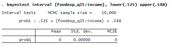
The estimated posterior probability is 0, which suggests that the effect of income on food expenditure differs between the 25th and 50th percentiles.