FITTING A MODEL TO SINGLE-RECORD-PER-EVENT INTERVAL-CENSORED DATA
Consider a fictional dataset simulated based on the Atherosclerosis Risk in Communities (ARIC) study described in Xu, Zeng, and Lin (2023). This dataset comprises 200 subjects, each from one of four US communities. The participants were followed over time and assessed for both diabetes and hypertension during several follow-up examinations. Because the subjects were examined only periodically, the exact onset times of these diseases were not observed, but they are known to fall in intervals between doctor visits. Two variables, ltime and rtime, capture this information by recording the last examination time before the event occurred and the first examination time after the event, respectively.
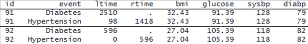
We wish to identify the factors that influence the times to onset of diabetes and hypertension. The factors of interest include three demographic variables—race, sex (male), and community—and five baseline risk factors: age (age), body mass index (bmi), glucose level (glucose), systolic blood pressure (sysbp), and diastolic blood pressure (diabp). The dataset contains one record per event per subject with the event-time information recorded as interval data. This type of data is called single-record-per-event interval-censored data. Here is a subset of the dataset for subjects 91 and 92:
. webuse aric
(Simulated ARIC data)

. format bmi glucose %6.2f

. list id event ltime rtime bmi - diabp if id==91 | id==92, sepby(id) noobs
We can fit a marginal Cox proportional hazards model in which the times to onset of diabetes and hypertension depend on the above factors of interest. In a single-record-per-event format, we must specify the id(), event(), and interval() options. The command performs intensive computations and may take a little longer to run.
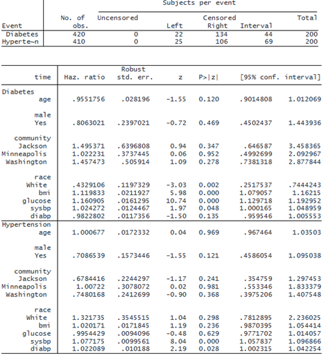
. stmgintcox age i.male i.community i.race bmi glucose sysbp diabp, id(id)
     event(event) interval(ltime rtime)
note: using adaptive step size to compute derivatives.

Performing EM optimization for event "Diabetes" (showing every 100 iterations):
Iteration 0:   Log pseudolikelihood = -179.18329
Iteration 100: Log pseudolikelihood = -110.21215
Iteration 200: Log pseudolikelihood = -109.98083
Iteration 300: Log pseudolikelihood = -109.93752
Iteration 400: Log pseudolikelihood = -109.92532
Iteration 500: Log pseudolikelihood = -109.92091
Iteration 600: Log pseudolikelihood = -109.91902
Iteration 624: Log pseudolikelihood = -109.91874

Performing EM optimization for event "Hypertension" (showing every 100 iterations):
Iteration 0:   Log pseudolikelihood = -208.75033
Iteration 100: Log pseudolikelihood = -160.09944
Iteration 200: Log pseudolikelihood = -159.88744
Iteration 300: Log pseudolikelihood =  -159.8376
Iteration 400: Log pseudolikelihood = -159.82201
Iteration 500: Log pseudolikelihood =  -159.8162
Iteration 600: Log pseudolikelihood = -159.81368
Iteration 610: Log pseudolikelihood = -159.81352

Computing standard errors: .....................................................
> ..............................................................................
> ..............................................................................
> ..............................................................................
> ..............................................................................
> ..............................................................................
> ........................... done

Marginal interval-censored Cox regression          Number of events   =      2
Baseline hazard: Reduced intervals                 Number of subjects =    200
                                                   Number of obs      =    400
ID variable: id                                            Uncensored =      0
Event variable: event                                   Left-censored =     47
Event-time interval:                                   Right-censored =    240
  Lower endpoint: ltime                                Interval-cens. =    113
  Upper endpoint: rtime
                                                   Wald chi2(20)      = 128.31
Log pseudolikelihood = -269.73225                  Prob > chi2        = 0.0000
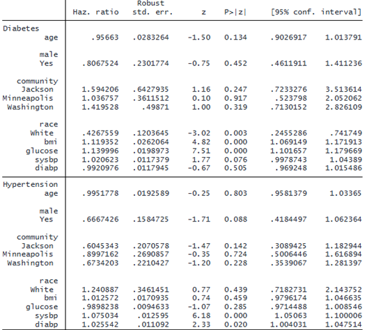
Note: Standard error estimates may be more variable for small datasets and
      datasets with low proportions of interval-censored observations.
The header above the coefficient table gives a summary of the censoring information. In the diabetes output, we notice that White individuals have a lower risk of diabetes. Additionally, higher body mass index and elevated glucose levels are associated with a higher risk of diabetes. In the output for hypertension, we see that higher systolic and diastolic blood pressure are associated with a greater risk of hypertension.
FITTING A MODEL WITH EVENT-SPECIFIC COVARIATES
From the model above, we can see that body mass index and glucose level are key risk factors for diabetes but not for hypertension. On the flip side, systolic and diastolic blood pressure appear to be important factors for hypertension but not for diabetes. Therefore, we can use different sets of covariates to model these two events. We also use the nolog option to suppress iteration logs and the favorspeed option to speed up computation.
. stmgintcox ("Diabetes": age i.male i.community i.race bmi glucose)
     ("Hypertension": age i.male i.community i.race sysbp diabp), id(id)
     event(event) interval(ltime rtime) nolog favorspeed

note: using fixed step size with a multiplier of 5 to compute derivatives.
note: using EM and VCE tolerances of 0.0001.
note: option noemhsgtolerance assumed.

Marginal interval-censored Cox regression          Number of events   =      2
Baseline hazard: Reduced intervals                 Number of subjects =    200
                                                   Number of obs      =    400
ID variable: id                                            Uncensored =      0
Event variable: event                                   Left-censored =     47
Event-time interval:                                   Right-censored =    240
  Lower endpoint: ltime                                Interval-cens. =    113
  Upper endpoint: rtime
                                                   Wald chi2(16)      =  77.01
Log pseudolikelihood = -272.76543                  Prob > chi2        = 0.0000
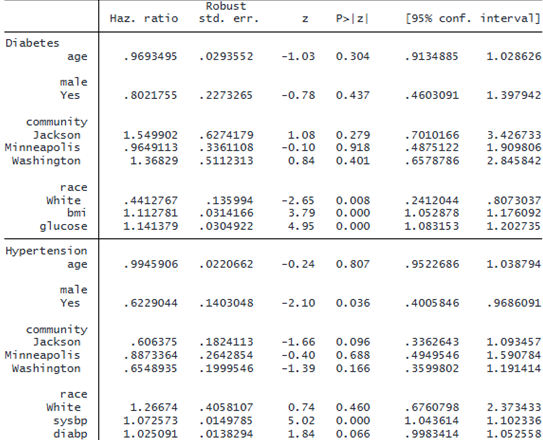
Note: Standard error estimates may be more variable for small datasets and
      datasets with low proportions of interval-censored observations.
Because age, male, community, and race are common covariates for both events, we can also specify the model by using a combination of common covariates and event-specific covariates:
. stmgintcox age i.male i.community i.race ("Diabetes": bmi glucose) ("Hypertension": sysbp diabp),
     id(id) event(event) interval(ltime rtime) nolog favorspeed
Both of the above specifications will give us the same result.
ESTIMATING AND TESTING THE COMMON EFFECT OF A COVARIATE ACROSS ALL EVENTS
After fitting the above model, suppose we want to test the hypothesis that the effects of age are zero for all events. We can use the estat common command to estimate an optimal weighted average effect of age across all events and conduct a z test to determine whether this average effect is zero under the null hypothesis.
© Copyright 1996–2026 StataCorp LLC. All rights reserved.
. estat common age

    _avg_age: .294*["Diabetes"]age + .706*["Hypertension"]age

We fail to reject the null hypothesis that the weighted average effect of age across all events is zero (the p-value is 0.518). When the effects are similar across different events, the average affect estimates the common effect, and this test is more powerful than the traditional multivariate Wald test, which can be performed with the test command.
GRAPHING SURVIVOR FUNCTIONS
We can use stcurve to plot the estimated survivor functions. By default, the stcurve command with the survival option evaluates the survivor functions at the overall means of covariates for each event and plots the survivor functions for both events as subgraphs.
. stcurve, survival
note: function evaluated at overall means of covariates for specified events.

We can add the sepevents option to request that the estimated survivor function for each event be displayed on a separate graph.
If we wish to compare the survival curve of an average person with diabetes across different communities, we can specify multiple values for community using the at() option and specify the event value label “Diabetes” in the events() option.
. stcurve, survival at(community=(1 2 3 4)) events("Diabetes")
note: function evaluated at specified values of selected covariates and
      overall means of other covariates (if any) for specified event.

The above survival curves show that an average person in Forsyth (blue line) and one in Minneapolis (green line) have a similar higher risk of developing diabetes, whereas an average person in Washington (yellow line) and one in Jackson (red line) have a lower risk of developing diabetes.
ASSESSING OVERALL MODEL FIT WITH GOODNESS-OF-FIT PLOTS
We can use the estat gofplot command to produce the event-specific goodness-of-fit plots and visually assess the overall model fit. estat gofplot calculates an empirical estimate of the cumulative hazard function based on the Cox–Snell-like residuals for each event and plots the resulting cumulative hazard rate against the residuals themselves. If the model fits the data, those plots are expected to remain close to the reference line.
. estat gofplot

By default, estat gofplot displays all event-specific goodness-of-fit plots as subgraphs within a single graph. The plot on the left indicates that the marginal Cox proportional hazards model fits the data well for diabetes. The plot on the right suggests that the marginal Cox model fits the data mostly well for hypertension, except for the tail, which deviates from the reference line because of an outlier.
FITTING A MODEL TO MULTIPLE-RECORD-PER-EVENT INTERVAL-CENSORED DATA
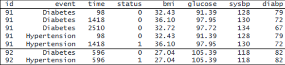
Interval-censored data can also be recorded in multiple-record-per-event format. In this format, each event for a subject may contain multiple records with multiple examination times and potential TVCs at each examination time. Here we use an extended version of the previous dataset. It contains all the baseline covariates as well as four time-varying covariates: bmi, glucose, sysbp, and diabp. It also records the examination time (time) and whether the event occurred since the last examination (status). Here is a subset of this dataset for subjects 91 and 92:
. webuse aric2
(Simulated ARIC data with time-varying variables)

. format bmi glucose %6.2f

. list id event time status bmi-diabp if id==91 | id==92, sepby(id) noobs
We use stmgintcox to fit a marginal Cox proportional hazards model in which the times to onset of events (diabetes and hypertension) depend on baseline covariates age, male, community, and race and TVCs bmi, glucose, sysbp, and diabp. In a multiple-record-per-event format, we must specify the id(), event(), time(), and status() options. We also include the detail option to get detailed censoring information for each event.
. stmgintcox age i.male i.community i.race bmi glucose sysbp diabp, id(id)
     event(event) time(time) status(status) detail nolog

note: time-varying covariates detected in the data; using method nearleft to
      impute their values between examination times.
note: using adaptive step size to compute derivatives.

Marginal interval-censored Cox regression        Number of events   =        2
Baseline hazard: Reduced intervals               Number of subjects =      200
                                                 Number of obs      =      830
ID variable: id                                          Uncensored =        0
Event variable: event                                 Left-censored =       47
Examination time: time                               Right-censored =      240
Status indicator: status                             Interval-cens. =      113

                                                 Wald chi2(20)      = 13197.36
Log pseudolikelihood = -264.77802                Prob > chi2        =   0.0000
Time varying: bmi glucose sysbp diabp
Note: Standard error estimates may be more variable for small datasets and
      datasets with low proportions of interval-censored observations.
After accounting for time-varying risk factors, we see that elevated glucose levels, a higher body mass index, and elevated systolic blood pressure are associated with an increased risk of diabetes onset. Race White is associated with a lower risk of developing diabetes. Also, elevated systolic and diastolic blood pressure levels are associated with a higher risk of developing hypertension.