OVERVIEW
When we use linear regression, we model the mean of the outcome. Yet, sometimes, we would like to study features of the outcome distribution other than the mean. For example, a policymaker may want to learn how participation in a 401(k) retirement plan would affect the lower-level, median, and upper-level conditional quantiles of net wealth.
ivqregress estimates parameters at quantiles of the outcome distribution and accounts for endogeneity problems that arise for reasons such as self-selection, omission of a relevant variable, or measurement error. For example, participation in the 401(k) program may be endogenous because the people who do and do not participate may have different saving preferences, which will affect net wealth growth.
WHEN QUANTILE REGRESSION MATTERS
Suppose we have a simple model E(y|x)=β0+xβ1, where yis the outcome variable and x is a covariate. xtakes values in {0,1,2,3,4,5,6}. By definition, β1 fully characterizes the effects of increasing one unit of xon the conditional mean of outcome y; that is, β1=E(y|x=a+1)−E(y|x=a). Below, we consider two scenarios of the data-generating process.
1. Location shifted only. The probability density function of the outcome conditional on x=a+1, f(y|x=a+1), is only location shifted relative to f(y|x=a). In this case, β1 summarizes the effect of xnot only on the conditional mean but also on each conditional quantile of y. This case is illustrated in the left panel of Figure 1.
2. Location shifted and rescaled. The probability density function of the outcome conditional on x=a+1, f(y|x=a+1), is both location shifted and rescaled relative to f(y|x=a). In this case, β1 summarizes the effect of x only on the conditional mean but not on the conditional quantiles of y. This case is illustrated in the right panel of Figure 1.
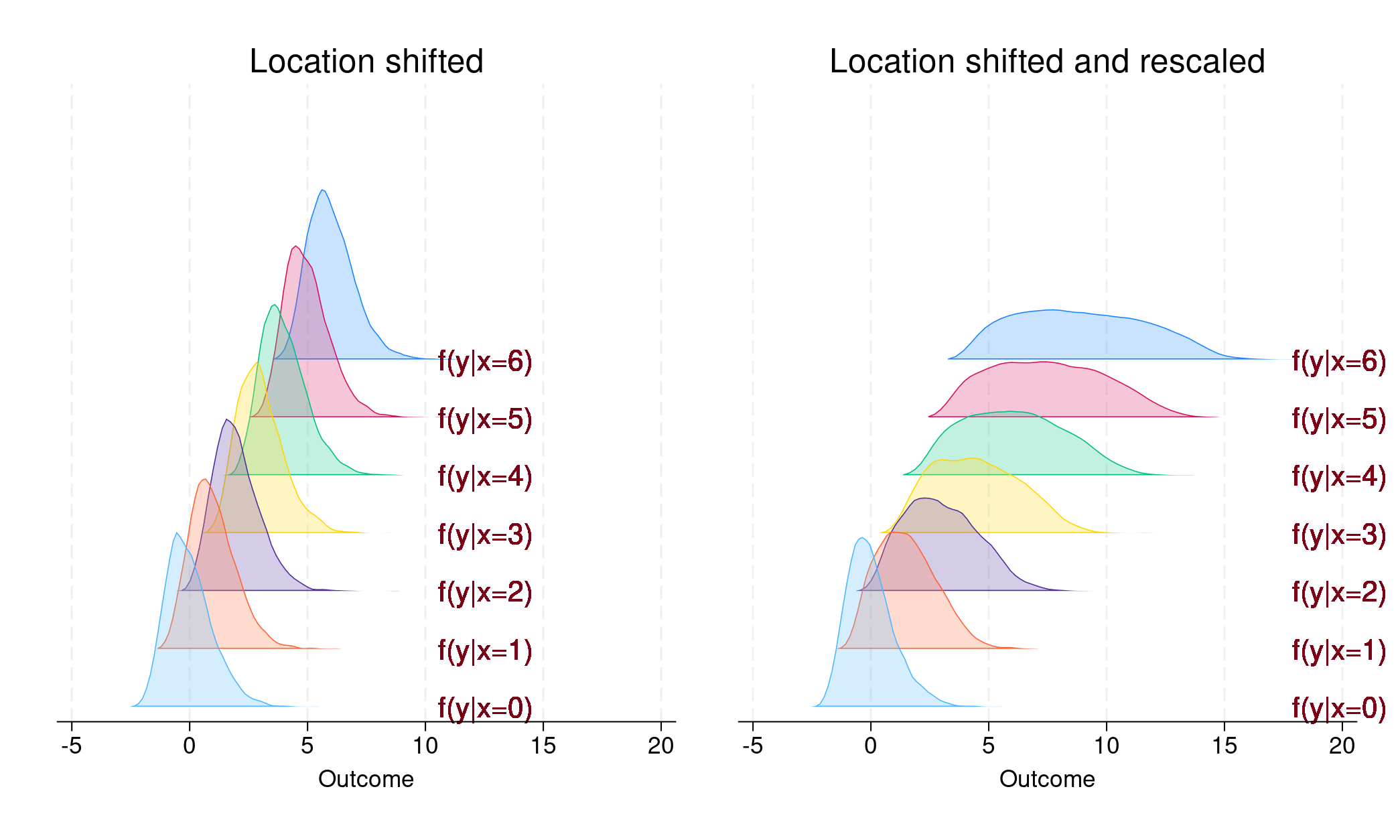 In the left panel, we see that each conditional density is parallel relative to the others; only the location has been shifted. In this case, β1 captures the shift in both conditional mean and any other conditional quantiles of the outcome. As a result, running a linear regression provides as much information about β1 as a quantile regression.
In contrast, in the right panel, the conditional density for each level of x has a different location and a different shape. Thus, β1 can summarize the shifts in conditional mean, which generally differ from the shifts in conditional quantiles. Quantile regression becomes necessary to learn about the effects of x on the conditional quantiles of the outcome.
INSTRUMENTAL-VARIABLES QUANTILE REGRESSION IN ACTION!
We want to estimate the effect of 401(k) participation (p401k) on different conditional quantiles of net financial assets (assets). We use data reported by Chernozhukov and Hansen (2004). These data are from a sample of households in the 1990 Survey of Income and Program Participation (SIPP). For the head of household, we have data on income (income), age (age), number of people in the family (familysize), marital status (married), participation in IRA (ira), participation in pension benefit (pension), home ownership (ownhome), and years of education (educ).
We suspect 401(k) participation is endogenous because it may depend on unobserved factors such as saving preference that also impact financial assets. We will use 401(k) eligibility (e401k) as an instrument for 401(k) participation.
We use the IQR estimator (ivqregress iqr) to estimate the effect of 401(k) participation on the conditional median (the default) of the net financial assets.
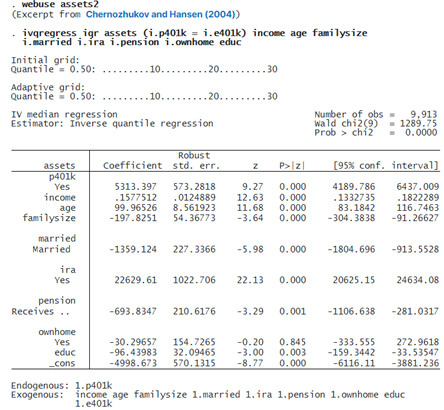
The coefficient for p401k is 5,313. This means participation in a 401(k) would increase the median net financial assets by $5,313, conditional on other covariates, relative to a scenario where no one participates.
After ivqregress iqr, we can use estat dualci to obtain the dual confidence interval (CI) that is robust to weak instruments for the coefficient on the endogenous variables.
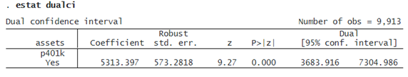
The dual CI is usually wider than the regular CI; it provides more robust inference if the instruments are weak. Here the dual 95% CI is [3684, 7305], which is wider than the regular 95% CI [4190, 6437].
© Copyright 1996–2024 StataCorp LLC. All rights reserved.
We have estimated the 401(k) participation (p401k) treatment effect on the conditional median of net financial assets (assets). However, from the policy designer’s point of view, we may be more interested in estimating the treatment effect of p401k on other conditional quantiles of assets.
This time, we specify ivqregress smooth to use the smoothed estimating equations estimator to fit the model at different quantiles. In particular, we specify the quantile(10(10)90) option to fit the IVQR model at the 10th, 20th, . . . , 90th quantiles.
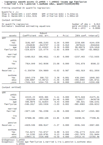
The results show the estimates for the effect of 401(k) participation on each conditional quantile of the asset. The coefficient interpretation is similar to before, except we are looking at different conditional quantiles. For example, for quantile q90, the estimate for the coefficient on p401k is 15,525. Thus, 401(k) participation would increase net financial assets’ 90% conditional quantile by $15,525.
In addition to looking at the exact numerical estimates from the coefficient table, we can use estat coefplot to visualize the p401k‘s treatment effect from the lower to the upper quantile.
. estat coefplot
 The dots in the plot show the point estimates of p401k‘s treatment effect on different conditional quantiles of assets, and the gray bound shows the 95% pointwise CI. We see an upward trend of p401k‘s treatment effect. At lower-level quantiles such as the 10th, 20th, 30th, and 40th quantiles, the treatment effect is relatively flat. However, the treatment effect increases in the upper-level quantiles. The red line shows the two-stage least-squares estimates, which can be used as a benchmark.
We can use estat endogeffects to test the following hypotheses regarding the endogenous covariate:
-
No effect : The 401(k) participation does not affect net financial assets for all the estimated quantiles.
-
Constant effect : The 401(k) participation’s treatment effect is constant for all the estimated quantiles.
-
Dominance : The 401(k) participation is unambiguously positive for all the estimated quantiles; that is, the coefficient values are strictly positive.
-
Exogeneity : The 401(k) participation is exogenous.
We use estat endogeffects to show the Kolmogorov–Smirnov statistic and the 95% critical value for each hypothesis. We can reject the null hypothesis if the test statistic is greater than the critical value; otherwise, we cannot reject the null hypothesis. We specify the rseed() option to make the results reproducible because the critical values are generated from a bootstrap sample.
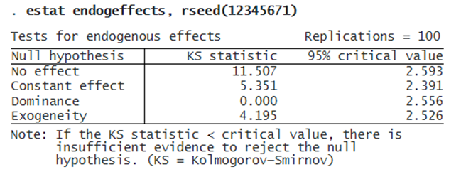
We find that 401(k) participation has some effect, treatment is not constant across different quantiles, and 401(k) participation is endogenous. The test for dominance indicates that 401(k) participation is unambiguously beneficial for all the estimated quantiles of assets.
The test results are consistent with the coefficient plot produced by estat coefplot, where we saw that the treatment effects are positive (dominance and no effect hypotheses) and upward trended (constant effect hypothesis).