ESTIMATION OF FLEXIBLE DEMAND SYSTEMS IN ACTION!

We have data from the Nationwide Food Consumption Survey, and we would like to estimate a demand system for a basket of goods that includes five food categories: dairy products, proteins, fruits and vegetables, flour-based products, and a miscellaneous category with all other food products. The observed data are at the household level. We have variables recording the total expenditure a household spends on food, the share spent on each food category, and the unit price for each food category. The budget shares of all food categories need to sum up to one. This is a typical data structure required for most demand systems. If needed, these variables can be constructed from the quantity purchased and dollar amount paid by the households.

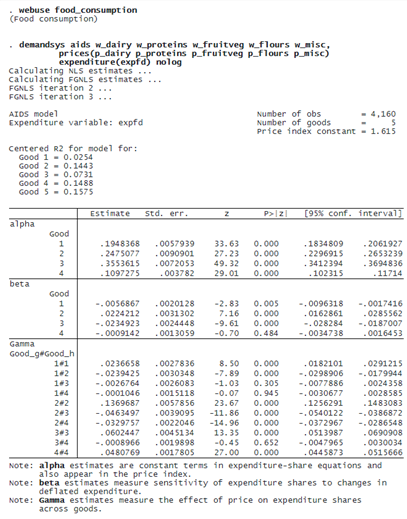
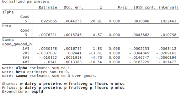
Let’s load the dataset and fit the AIDS model:

Usually, we do not interpret the above estimated parameters directly; instead, we use them to compute elasticities. We will see some examples of this below.

We might suspect a nonlinear relationship when the Engel curves (relationship between expenditure and income) have a quadratic representation. In the demand system world, we can examine the relationship between the budget share and expenditure:

. generate lnexp = ln(expfd)
. twoway (qfitci w_dairy lnexp), ylabel(,format(%5.2f))   
  ytitle("Budget share") xtitle("Log of expenditure")                         
  title("Nonlinear relationship for dairy products")

Because of the quadratic representation, we might consider the QUAIDS model, which includes the quadratic term of expenditure with respect to the budget shares. Below, we fit a QUAIDS model and we include two demographic variables that also affect demand, the number of children, and the number of adults in the household.

© Copyright 1996–2024 StataCorp LLC. All rights reserved.

These variables are specified in the demographics() option, and they can be included in the model via demographic translation (Pollak and Wales 1978) or demographic scaling (Ray 1983; Poi 2002). We use demographic translation.

. demandsys quaids w_dairy w_proteins w_fruitveg w_flours w_misc, 
            prices(p_dairy p_proteins p_fruitveg p_flours p_misc) 
	    expenditure(expfd) nolog demographics(n_kids n_adults)

(output omitted)

Previously, we created a scatterplot to assess whether there might be a quadratic relationship. To provide statistical evidence of this relationship, we perform a joint test on all the coefficients associated with the quadratic terms:

. test [lambda]1.Good [lambda]2.Good [lambda]3.Good [lambda]4.Good

 ( 1)  [lambda]1bn.Good = 0
 ( 2)  [lambda]2.Good = 0
 ( 3)  [lambda]3.Good = 0
 ( 4)  [lambda]4.Good = 0

           chi2(  4) =   17.21
	 Prob > chi2 =    0.0018

The goal of fitting a demand system is to compute the elasticities, which requires the parameter estimates and data. The postestimation tools for demandsys make elasticities easy to compute.

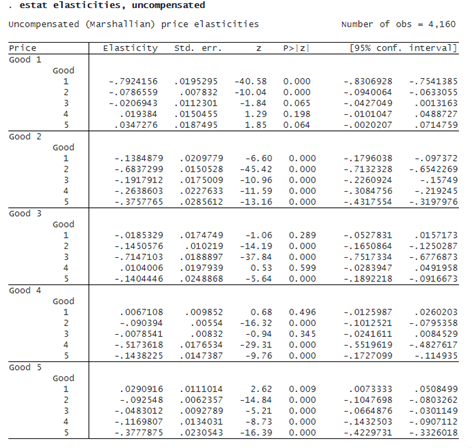
To compute the uncompensated own-price and cross-price elasticities, we type

All the own-price elasticities fall above –1, and they range from –.7924 to –.3778. These values indicate that there is an inelastic demand for food products; we also see that some goods are complements for others, and others are substitutes. Above, we requested uncompensated elasticities; if we instead want compensated elasticities, we can specify the compensated option instead of uncompensated; compensated elasticities are smaller in absolute terms because they contain only substitution effects, while uncompensated elasticities also account for income effects.

Suppose we are also interested in the expenditure elasticities for households with two kids. We use the expenditure option to obtain expenditure elasticities and use the if qualifier to restrict the sample to these households:

All the expenditure elasticities are obtained at sample means, and they are close to 1. Without the transition from expenditure to income, we cannot really say whether they are normal or luxury goods, but the results shed light on how sensitive households are to expenditure changes when it comes to food consumption given the observed data.