Panel-data multinomial logit model
The multinomial logit (MNL) model is a popular method for modeling categorical outcomes that have no natural ordering—outcomes such as occupation, political party, or restaurant choice.
In longitudinal/panel data, we observe a sequence of outcomes over time. Say that we observe restaurant choices made by individuals each week. Do you think that restaurant choices are independent from week to week? Probably not. Someone who likes Italian food is likely to choose an Italian restaurant multiple times. These choices are driven by underlying personal preferences and characteristics, some of which are not observed.
Stata’s new xtmlogit command fits random-effects and conditional fixed-effects MNL models for categorical outcomes observed over time.
To fit a random-effects multinomial logit model, we can type
. xtset subject
. xtmlogit restaurant age
and estimate the standard multinomial logit coefficients accounting for time-invariant subject-specific characteristics by including random effects specific to each outcome level.
With the command above, the random effects are assumed to be normally distributed and independent across outcome levels (restaurant choices), but several variance–covariance structures are supported, including a completely unrestricted covariance:
. xtmlogit restaurant age, covariance(unstructured)
If you suspect that subject-specific effects might be correlated with age, you can use a conditional fixed-effects estimator to account for this:
. xtmlogit restaurant age, fe
Let’s see it work
We wish to find out whether individuals are more likely to be out of the labor force if they have children under the age of five in their household. We will use a (fictitious) dataset of men and women who were asked about their employment status every two years.
. use https://www.stata-press.com/data/r17/estatus
(Fictitious employment status data)
Here is an excerpt of the dataset, showing the employment history for three individuals:
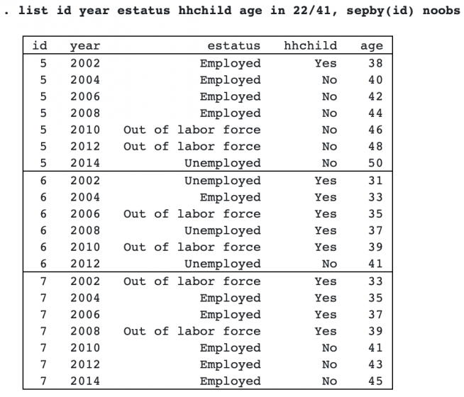
The outcome of interest is employment status (estatus), which has three levels: Employed, Unemployed (but seeking employment), and Out of labor force (not seeking employment). Our predictor of interest, hhchild, indicates whether they have children under the age of five in their household at the time of the interview.
Before we can fit our model, we need to specify our panel identifier variable, id, by using xtset.
. xtset id

Panel variable: id (unbalanced)
Now we can use xtmlogit to model the probability of each employment type by hhchild while controlling for the effects of age, annual household income (hhincome), and whether a significant other was also living in the household (hhsigno). We will start with a random-effects model (the default) and use the rrr option to get exponentiated coefficients that can be interpreted as relative-risk ratios.
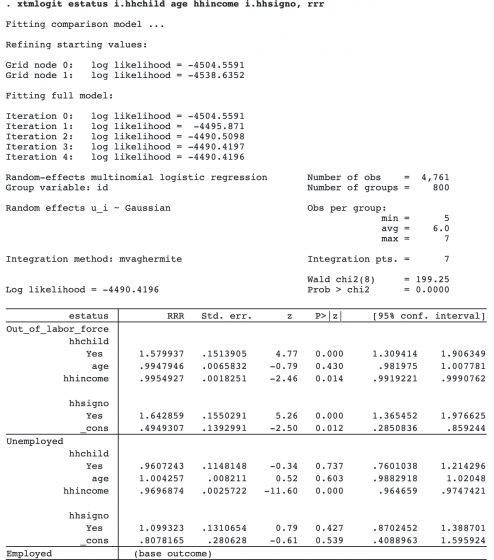
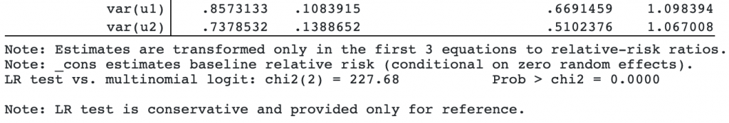
The first two sections in the output show the relative-risk ratio estimates of our predictors with respect to the base category Employed. The last section shows the estimated variances of the random effects. By default, the random effects are uncorrelated, but their covariance structure can be changed using the covariance() option. For example, correlations between random effects can be estimated using covariance(unstructured), or each category can share a common random effect using covariance(shared).
Adjusting for age, household income, and having a significant other at home, the relative risk of being out of the labor force for individuals having at least one child under the age of 5 in the household versus having no children under 5 in the household is 1.6 times as large as the relative risk of employment (95% CI [1.3, 1.9]). To understand these effects in terms of probabilities, we can use the margins command.
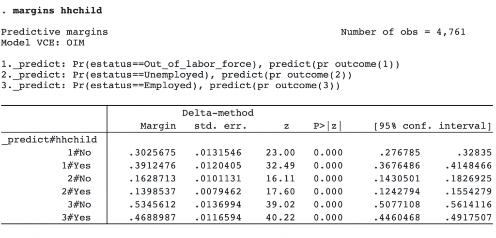
For an individual without children, the expected probability of being out of the labor force (labeled 1#No) is 0.30, the expected probability of being unemployed (2#No) is 0.16, and the expected probability of being employed is 0.53 (3#No). We also find that individuals with children in the household increase their probability of being out of the labor force by 9 percentage points. We could see how these probabilities change by household income using an additional margins command and visualize the results using marginsplot.
. quietly margins hhchild, at(hhincome=(20(20)100))

. marginsplot, by(_predict, label("Out of labor force" "Unemployed" "Employed"))
byopts(rows(1) title("Marginal probabilities of employment status"))
legend(order(4 "Child under 5 at home" 3 "No child under 5 at home"))

To get separate graphs for each outcome, we used the by(_predict) option in marginsplot. The rest of the options add titles and labels.
Comparing the lines within each employment category, we see that having a child at home does not have much impact on the probability of being unemployed but does influence the decision to work or to be out of the labor force.
In the model we just fit, we used random effects to account for unobserved characteristics of the individuals in our dataset. Random-effects models require that the random effects be uncorrelated with the predictors, and the random-effects MNL model is no exception. A widely used alternative is the fixed-effects estimator. To fit our model with conditional fixed effects, we simply add the fe option.
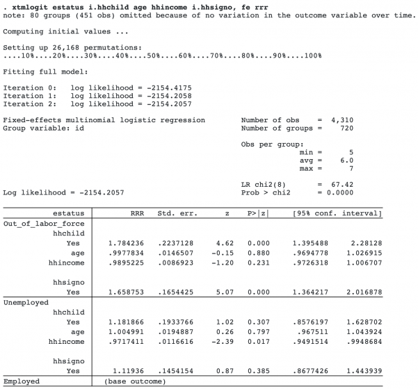
The results are similar to those of the random-effects estimator. And they can be interpreted in the same way.