LISREL is a 64-bit application for standard and multilevel structural equation modeling. These methods are available for the complete and incomplete complex survey data on categorical and continuous variables as well as complete and incomplete simple random sample data on categorical and continuous variables.

MULTILEV is a 64-bit application that fits multilevel linear and nonlinear models to multilevel data from simple random and complex survey designs. It allows for models with continuous and categorical response variables.

MGLIM is a 64-bit application that uses adaptive quadrature to fit generalized linear models with categorical, count and non-normally distributed outcome variables to multilevel data.

SURVEYGLIM is a 64-bit application that fits Generalized LInear Models (GLIMs) to data from simple random and complex survey designs. Models for the Multinomial, Bernoulli, Binomial, Negative Binomial, Poisson, Normal, Gamma, and Inverse Gaussian sampling distributions are available.

CONTINUOUS VARIABLES

MOMENT MATRICES

Suppose that the rows of X (n x p) are n observations of p continuous variables x1, x2,…,  xp with mean vector μ  and covariance matrix Σ . The sample covariance matrix, S , is an unbiased estimator of Σ and may be expressed as

where xi and ¯x denote observation i and the sample mean vector of x = , respectively. A typical element of a consistent estimator, U, of the asymptotic covariance matrix,ϒ, of the sample variances and covariances (Browne 1984) is given by

The robust ML, DWLS, WLS, and ULS methods can be used to fit structural equation models for continuous variables to the sample covariance matrix by using the estimated asymptotic covariance matrix of the sample variances and covariances.

The correlation matrix, P, x1, x2,…,  xp is the covariance matrix of the standardized variables z1, z2,…,  zp where

and

where Dσ denotes a diagonal matrix with the standard deviations σ1,σ2,…, σp of x1, x2,…,  xp on the diagonal. The sample correlation matrix, R, is an unbiased estimator of P and may be expressed as

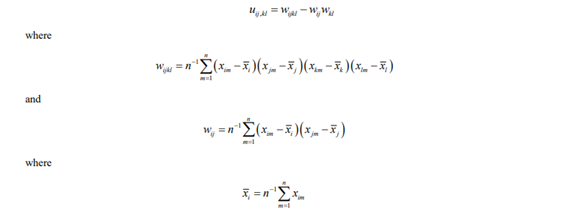
where Ds denotes a diagonal matrix with the sample standard deviations s1,s2,…, sp of x1,x2,…, xp on the diagonal. A typical element of a consistent estimator, U, of the asymptotic covariance matrix, ϒ, of the sample correlations (Steiger and Hakstian 1982) is given by

where

and

and

The robust DWLS, WLS, and ULS methods can be used to fit structural equation models for continuous variables to the sample correlation matrix by using the estimated asymptotic covariance matrix of the sample correlations.

MULTIPLE IMPUTATION

The MCMC method

Suppose now that the n observations of the p continuous variables include missing data values with k missing data value patterns and that the joint distribution of the variables is a multivariate normal distribution with mean vector μ and covariance matrix Σ.  The EM algorithm and the MCMC method for multiple imputation of incomplete data can be used to impute the missing data values of the continuous variables.

Suppose that Xo denote the observed data values. The EM algorithm (Dempster, Laird, and Rubin 1977) can be used to compute the maximum likelihood estimate of Σ. The minus two observed-data log likelihood may be expressed as

where ni denotes the number of observations of missing data value pattern i = 1,2,…, k, Σi denotes the population covariance matrix of missing data value pattern i, μi denotes the mean vector of missing data value pattern i, and xoij is the jth vector of observed values of missing data value pattern i.

The initial estimate for the M-step is the sample covariance matrix, S, of the complete data or Ip if the number of complete observations is too small. In the E-step, the conditional covariance matrices of the missing variables given the observed variables of the missing data value patterns are computed and used to compute an updated estimate  of Σ. Iteration of the consecutive M and E steps is terminated when the absolute difference between  and  is below the tolerance limit ε = 10-5.

The EM estimate, Σˆ, of Σ is used as the initial covariance matrix of the multivariate normal distribution in the first step of the Monte Carlo Markov Chain (MCMC) method. In the first step (P-step) of the MCMC method, an estimate of Σ is simulated from an inverse Wishart distribution. In the I-step, observations are simulated from the conditional normal distributions of the missing variables given the observed k missing data value patterns and used to replace the missing data values. The next estimate of Σ is then obtained by computing the sample covariance matrix of the completed data. The P and I steps are repeated for a fixed number of times.

The FCS regression method

Suppose now that the n observations of the p continuous variables include missing data values and that a joint (multivariate) distribution of the variables exists. In this case, the Fully Conditional Specified (FCS) regression method (Brand 1999; Van Buuren 2007) can be used to impute the missing data values. The FCS regression method performs a fixed number of imputations to impute the missing data values. Each imputation consists of a filled-in phase and an imputation phase. In the filled-in phase, the missing data values are filled-in by using a sequence of regression analyses for the p continuous variables. These filled-in data are then used as the initial data for the imputation phase in which the missing data values are imputed by using a sequence of regression analyses for the p continuous variables. These imputed data are then used as the initial data for the next iteration of the imputation phase and a fixed number of iterations are executed for each imputation.

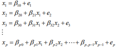
The filled-in stage fits the following p regression models sequentially to the data, namely

where the elements of β = denote unknown regression weights and e1,e2,…, ep are p error variables. The first model is fitted to the complete data for x1. The corresponding estimates are then used to simulate new parameter values from the posterior distributions of the parameters which in turn is used to fill-in the missing data values for x1. The second model is then fitted to the complete data for x2 and the filled-in data for x1. The final model is fitted to the complete data for xp and the filled-in data for x1,x2,…, xp-1. The filled-in data for x1,x2,…, xp are used for the first iteration of the imputation phase. The simulation of the new parameter values from the posterior distributions of the parameters and the imputation of the missing data values for each of the p regression models use the same steps as outlined next for each iteration of the imputation stage.

For each iteration of the imputation stage, the following regression models are fitted sequentially either to the filled-in data or the imputed data, namely

where j = 1,2,…, p, the elements of βj =  denote p unknown regression weights, and ej denotes an error variable with variance σ²j. The estimated covariance matrix of the estimator βjˆ of βj may be expressed as

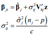
where X(j) denotes rows 1,2,…, j-1, j,…, p of the filled-in or imputed data. New values for the parameters are then simulated from their posterior distributions as

where Vhj denotes the upper triangular matrix in the Cholesky decomposition of Vj =V’hj Vhj, z denotes a p x 1 standard normal vector, and c is a Chi-square variable with nj – p degrees of freedom. The missing data values are then imputed as

where xijm denotes a missing data value in row i and column j of X, xi(j) denotes row i of X(j), and z is a standard normal variable.

Average unstandardized moment matrices

Suppose that X1,X2,…,Xm are m imputed data sets for the incomplete data matrix, X, of the p continuous variables x1,x2,…, xp and that S1,S2,…, Sm and U1,U2,…, Um denote the corresponding sample covariance matrices and the estimated asymptotic covariance matrices of the variances and covariances, respectively. Then, the average sample covariance matrix is

and the average estimated asymptotic covariance matrix is

Chung and Cai (2019) point out that Ū only captures uncertainty based on complete data. As a result, its inverse cannot be used as a weight matrix for the robust ML, DWLS, WLS, and ULS methods for continuous structural equational modeling. A corrected weight matrix is obtained by correcting for the between-imputation variation in the estimated variances and covariances and is obtained as the inverse of

where sdenotes the p x (p+1)/2 vector consisting of the nonduplicated elements of the p x p symmetric matrix S. S̄ and ϒ can be used to fit structural equation models to the average sample covariance matrix with the robust ML, DWLS, WLS, and ULS methods. The corrected robust DWLS and ULS Chi-square test statistic proposed by Chung and Cai (2019) is given by

where

where Δ denotes the Jacobian matrix of σ(θ) with respect to the unknown parameters θ of the structural equation model evaluated at θ=θ. The small sample adjusted Tb test statistic (Yuan and Bentler 1997) is given by

Average standardized moment matrices

Suppose that X1,X2,…,Xm are m imputed data sets for the incomplete data matrix, X, of the p continuous variables x1,x2,…, xp and that R1,R2,…, Rm and U1,U2,…, Um denote the corresponding sample correlation matrices and the estimated asymptotic covariance matrices of the sample correlations, respectively. Then, the average sample correlation matrix is

and the average estimated asymptotic covariance matrix is

Chung and Cai (2019) point out that Ū only captures uncertainty based on complete data. As a result, its inverse cannot be used as a weight matrix for the robust DWLS, WLS, and ULS methods for continuous structural equational modeling for correlation matrices. A corrected weight matrix is obtained by correcting for the between-imputation variation in the estimated correlations and is obtained as the inverse of

where r denotes the p x (p-1)/2 vector consisting of the nondiagonal and the nonduplicated elements of the p x p symmetric matrix R. R̄ and ϒ can be used to fit structural equation models to the average sample correlation matrix with the robust DWLS, WLS, and ULS methods. The corrected robust DWLS and ULS Chi-square test statistic proposed by Chung and Cai (2019) is given by

where

where Δ denotes the Jacobian matrix of p (θ) with respect to the unknown parameters θ of the structural equation model evaluated at θ=θ. The small sample adjusted Tb test statistic (Yuan and Bentler 1997) is given by

ORDINAL VARIABLES

Polychoric Correlations

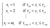
Suppose that the rows of X (nxp) are n observations of p ordinal variables x1,x2,…, xp with m1,m2,…, mp categories, respectively. Suppose further that these p ordinal variables are the result of the discretization of the underlying p  continuous standard normal variables z1,z2,…, zp as such that z =  ∼ N (0,P) and

where P denotes the population correlation matrix of z and are parameters known as thresholds. The model for the univariate marginal of variable xi is

where ∅ (.) denotes the probability density function of the standard normal distribution. The maximum likelihood estimator of  (Jöreskog, 1994) is given by

where Φ -¹ denotes the inverse of the cumulative distribution function of the standard normal distribution and pi1, pi2,…, pimi denote the marginal sample proportions for xi.

The polychoric correlation matrix, R, is a consistent estimator of the population correlation matrix P. The model for the bivariate marginal of variables xi and xj is

where ∅2 (u,v, pij) denotes the probability density function of the bivariate standard normal distribution with correlation pij. The maximization of the bivariate likelihood function is equivalent to minimization of the discrepancy function

where  and  denote the maximum likelihood estimators of the mi – 1 and mj – 1 thresholds of variables xi and xj, respectively and is the sample proportion for xi = k and xj = l. The gradient of F (.) (Olsson 1979) may be expressed as

where (Olsson 1979)

where ∅2 (.)  denotes the density function of the bivariate standard normal distribution with correlation pij. The information (Jöreskog, 1994) is given by

The Fisher scoring algorithm is used to minimize F (.) with respect to pij .  Let θ= pij . If  denotes the tth successive approximation to θ, then the (t + 1)st approximation is obtained from

Iteration is terminated when the absolute gradient value is below the tolerance limit ε=10-³.

The asymptotic covariance matrix, ϒ, of the p* = p(p-1)/2  polychoric correlations is a p*(p*+1)/2 matrix. A typical element of ϒ (Jöreskog, 1994) may be expressed as

where  and 0 otherwise   denotes a typical element of

where 1i denotes an mi x 1 column vector and

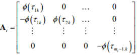
where Ai denotes the mi x (mi – 1) matrix given by

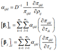
Typical elements of αij, βi, and βj are given by

where

The robust DWLS, WLS, or ULS methods can be used to fit structural equation models for ordinal variables to the polychoric correlation matrix by using the estimated asymptotic covariance matrix of the polychoric correlations (Chung and Cai (2019)).