| |
A Visual Guide to Stata Graphics, Third Edition - By Michael N. Mitchell Table of Contents

Dedication
Acknowledgments
Preface
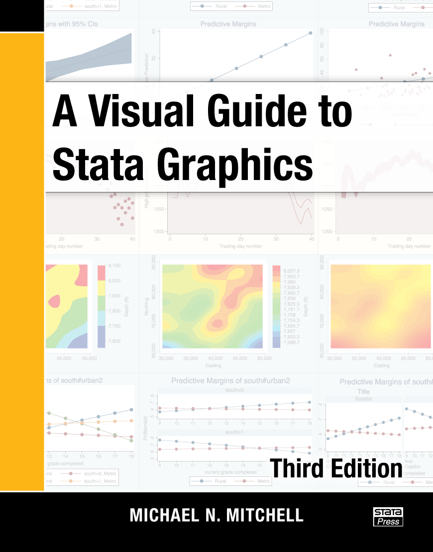
In its third edition, Michael Mitchell’s A Visual
Guide to Stata Graphics remains the essential introduction and
reference for Stata graphics. The third edition retains all the
features that made the first two editions so useful:
- A complete guide to Stata’s graph command and Graph Editor
- Exhaustive examples of customized graphs using both command options and the Graph Editor
- Visual indexing of features—just look for a picture that matches what you want to do
New in this edition are treatments of contour plots, margins
plots, and font handling. Mitchell dedicates a new subsection to
contour plots, showing you how to control the number of levels, how to
change the colors used, and how to produce effective legends. Over 30
graphs are used to demonstrate what you can accomplish with the new
marginsplot command—graphs of estimated means and marginal means (with
confidence intervals), interaction graphs, comparisons of groups, and
more. Mitchell also adds a section that shows you how to get bold text,
italic text, subscripts, superscripts, and Greek letters into your
titles, axes, labels, and other text.
The book retains its visual style, presenting the reader with a
color-coded, visual table of contents that runs along the right edge of
every page and shows readers exactly where they are in the book. You
can see the color-coded chapter tabs without opening the book,
providing quick visual access to each chapter.
The heart of each chapter is a series of entries that are typically
formatted three to a page. Each entry shows a graph command (with the
emphasized portion of the command highlighted in red), the resulting
graph, a description of what is being done, the dataset and scheme
used, and a section showing how to produce the result by using the
Graph Editor. Because every feature, option, and edit is demonstrated
with a graph or screen capture, you can often flip through a section of
the book to find exactly the effect you are seeking.
The first chapter details how to use the book, the types of Stata
graphs, how to use schemes to control the overall appearance of graphs,
and how to use options to make specific modifications. It also outlines
a process for building graphs with the graph command.
The second chapter is a complete overview of the Graph Editor. It
includes over 120 color graphics and screen captures to show exactly
how things are done and how they look on the graph. With pictures and
words, Mitchell shows how to change the color, size, or placement of
any titles, markers, annotations, or other objects on your graph by
using just a few mouse clicks. More subtly, he shows how to change
things such as the number of ticks and labels on your axes, the number
of columns in your legends, the label on an individual point, and more.
He even shows how to convert, for example, a scatterplot to a line plot
and how to rotate or pivot bar charts. Mitchell also covers advanced
topics such as how to draw lines and arrows on graphs so that they
continue to reference your objects of interest even if you resize the
graph, combine it with other graphs, or change the scale or range of
the axes. In short, he exposes all the Graph Editor’s tools, from the
simplest to the most powerful. Mitchell does not stop there; almost
every example in the book shows you how to accomplish the desired graph
or effect not only by using a command or command-line option but also
by using the Graph Editor.
Of the Graph Editor, Mitchell writes,
[...] You need to use the
Graph Editor for only a short amount of time to see what a smart and
powerful tool it is. Whereas commands offer the power of repeatability,
the Graph Editor provides a nimble interface that permits you to
tangibly modify graphs like a potter directly handling clay.
In the third chapter, Mitchell discusses twoway graphs such as
scatterplots, line plots, area plots, bar plots, range plots, contour
plots, regression fits, and smooths. He shows how to create each of
these types of graphs and how to use options (and the Graph Editor) to
control how the graph looks. He also introduces graphing across groups
of data and options for adding and controlling titles, notes, legends,
and so forth. Beyond the basics, he shows how to easily overlay plots
to obtain graphs such as regression fits with error contours and
observed data scatters, local polynomial smooths with scatters of their
underlying data, stock market–style graphs of open and closed values
with quantities traded as a bar chart at the bottom, histograms with
density smooths, and more. Because Stata’s graph command will let you
customize any aspect of the graph, Mitchell spends ample time showing
you the most valuable options for obtaining the look you want. If you
are in a hurry to discover one special option, you can skim the chapter
until you see the effect you want, and then glance at the command to
see what is highlighted in red.
In the succeeding five chapters, Mitchell covers scatterplot matrices,
bar graphs, box plots, dot plots, and pie charts. As with twoway
graphs, he shows you how to create each of these graphs and how to
adjust every aspect of the graph to your taste (or to a publisher’s
required form).
In chapters 9 and 10, Mitchell undertakes an in-depth presentation of
the options available across almost all graph types—options that add
and change the look of titles, notes, and such; control the number of
ticks on axes; control the content and appearance of the numbers and
labels on axes; control legends; add and change the look of
annotations; graph over subgroups; change the look of markers and their
labels; apply schemes to control the look of the graph; change the look
of graph regions; size graphs and their elements; and more. Again he
shows how to make these changes both by using options and by using the
Graph Editor.
To complete the graphical journey, Mitchell discusses and demonstrates
the 12 styles that unite and control the appearance of the myriad graph
objects. These styles are angles, colors, clock positions, compass
directions, connecting points, line patterns, line widths, margins,
marker sizes, orientations, marker symbols, and text sizes.
That completes the main body of the Visual Guide, but don’t skip the
appendix. There, Mitchell first gives a quick overview of the dozens of
statistical graph commands that are not strictly the subject of the
book. Even so, these commands use the graph command as an engine to
draw their graphs; therefore, almost all that Mitchell has discussed
applies to them. To make this clear, he shows explicitly how to apply
common options and common Graph Editor tools to statistical graphs.
Then Mitchell takes you on a tour of the new marginsplot command. After
that, he addresses combining graphs—showing you how to create complex
and multipart images from previously created graphs.
In a crucial section entitled “Putting it all together”, Mitchell shows
us how to do just that. We learn more about overlaying twoway plots,
and we learn how to combine data management and graphics to create
plots such as bar charts of rates with capped confidence intervals,
scatterplots with range-finder confidence intervals in both dimensions,
and population pyramids.
Mitchell then warns us about mistakes that can be made when typing
graph commands and how to correct them. In the appendix, he even show
us how to create our own scheme files. Scheme files allow you to
control every aspect of how your graphs look without having to specify
options. They are the answer to department or journal standards or if
you just want all your graphs to have a common appearance different
from the schemes shipped with Stata. As with the rest of the book, this
section includes cross-references to the Stata Graphics Reference
Manual to provide more depth on the subject. Finally, Mitchell reviews
all datasets, schemes, and other online supplements available for the
book.
The third edition of A Visual Guide to Stata Graphics is a complete
guide to Stata’s graph command and the associated Graph Editor. Whether
you want to tame the Stata graph command, quickly find out how to
produce a graphical effect, master the Stata Graph Editor, or learn
approaches that can be used to construct custom graphs, this is the
book to read.
Preface to the Third Edition
Preface to the Second Edition
Preface to the First Edition
- Introduction
- Using this book
- Types of Stata graphs
- Schemes
- Options
- Building graphs
- Editor
- Overview of the Graph Editor
- Object Browser
- Modifying objects
- Adding objects
- Moving objects
- Hiding and showing objects
- Locking and unlocking objects
- Using the Graph Recorder
- Graph Editor versus Stata commands
- Twoway Graphs
- Scatterplots
- Regression fits and splines
- Regression confidence intervals fits
- Line plots
- Area plots
- Bar plots
- Range plots
- Distribution plots
- Contour plots
- Options
- Overlaying plots
- Scatterplot Matrix Graphs
- Marker options
- Controlling axes
- Matrix options
- Graphing by groups
- Bar Graphs
- Y-variables
- Graphing bars over groups
- Options for controlling gaps between bars
- Options for sorting bars
- Controlling the categorical axis
- Legends and labeling bars
- Controlling the y-axis
- Changing the look of bars
- Graphing by groups
- Box Plots
- Specifying variables and groups
- Options for controlling gaps between boxes
- Options for sorting boxes
- Controlling the categorical axis
- Controlling legends
- Controlling the y-axis
- Changing the look of boxes
- Graphing by groups
- Dot Plots
- Specifying variables and groups
- Options for controlling gaps between dots
- Options for sorting dots
- Controlling the categorical axis
- Controlling legends
- Controlling the y-axis
- Changing the look of dot rulers
- Graphing by groups
- Pie Graphs
- Type of pie graphs
- Sorting pie slices
- Changing the look and color and exploding pie slices
- Slice labels
- Controlling legends
- Graphing by groups
- Options available for most graphs
- Changing the look of markers
- Creating and controlling marker labels
- Connecting points and markers
- Setting and controlling axis titles
- Setting and controlling axis labels
- Controlling axis scales
- Selecting an axis
- Graphing by groups
- Controlling legends
- Adding texts to markers and positions
- Options for text and textboxes
- More options for texts and text
- Standard options available for all graphs
- Creating and controlling titles
- Using schemes to control the look of graphs
- Sizing graphs and their elements
- Changing the look of graph regions
- Styles for changing the look of graphs
- Angles
- Colors
- Clock position
- Compass direction
- Connecting points
- Line patterns
- Line width
- Margins
- Marker size
- Orientation
- Marker symbols
- Text size
- Appendix
- Overview of stastistical graph commands
- Common options for statistical graphs
- The marginsplot command
- Saving, redisplaying, and combining graphs
- More examples: Putting it all together
- Common mistakes
- Customizing schemes
- Online supplements
Subject Index
© Copyright StataCorp LP 2002-2015.


|
|

