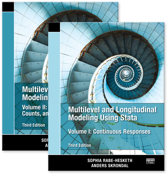
Multilevel and Longitudinal Modeling Using Stata, Third Edition
Volume I: Continuous Responses
Volume II: Categorical Responses, Counts, and Survival
by Sophia Rabe-Hesketh and Anders Skrondal

Multilevel and Longitudinal Modeling Using Stata, Third Edition,
by Sophia Rabe-Hesketh and Anders Skrondal, looks specifically at
Stata’s treatment of generalized linear mixed models, also known as
multilevel or hierarchical models. These models are “mixed” because
they allow fixed and random effects, and they are “generalized” because
they are appropriate for continuous Gaussian responses as well as
binary, count, and other types of limited dependent variables.
The material in the third edition consists of two volumes, a result of
the substantial expansion of material from the second edition, and has
much to offer readers of the earlier editions. The text has almost
doubled in length from the second edition and almost quadrupled in
length from the original version, to almost 1,000 pages across the two
volumes. Fully updated for Stata 12, the book has 5 new chapters, more
than 20 new exercises, and many new datasets.
The two volumes comprise 16 chapters organized into eight parts.
Volume I is devoted to continuous Gaussian linear mixed models and has
nine chapters organized into four parts. The first part reviews the
methods of linear regression. The second part provides in-depth
coverage of two-level models, the simplest extensions of a linear
regression model.
Rabe-Hesketh and Skrondal begin with the comparatively simple
random-intercept linear model without covariates, developing the mixed
model from principles and thereby familiarizing the reader with
terminology, summarizing and relating the widely used estimating
strategies, and providing historical perspective. Once the authors have
established the mixed-model foundation, they smoothly generalize to
random-intercept models with covariates and then to a discussion of the
various estimators (between, within, and random-effects). The authors
then discuss models with random coefficients.
The third part of volume I describes models for longitudinal and panel
data, including dynamic models, marginal models (a new chapter), and
growth-curve models (a new chapter). The fourth and final part covers
models with nested and crossed random effects, including a new chapter
describing in more detail higher-level nested models for continuous
outcomes.
The mixed-model foundation and the in-depth coverage of the mixed-model
principles provided in volume I for continuous outcomes make it
straightforward to transition to generalized linear mixed models for
noncontinuous outcomes, which are described in volume II.
Volume II is devoted to generalized linear mixed models for binary,
categorical, count, and survival outcomes. The second volume has seven
chapters also organized into four parts. The first three parts in
volume II cover models for categorical responses, including binary,
ordinal, and nominal (a new chapter); models for count data; and models
for survival data, including discrete-time and continuous-time (a new
chapter) survival responses. The fourth and final part in volume II
describes models with nested and crossed-random effects with an
emphasis on binary outcomes.
The book has extensive applications of generalized mixed models performed in Stata. Rabe-Hesketh and Skrondal developed gllamm,
a Stata program that can fit many latent-variable models, of which the
generalized linear mixed model is a special case. As of version 10,
Stata contains the xtmixed, xtmelogit, and xtmepoisson commands for fitting multilevel models, in addition to other xt
commands for fitting standard random-intercept models. The types of
models fit by these commands sometimes overlap; when this happens, the
authors highlight the differences in syntax, data organization, and
output for the two (or more) commands that can be used to fit the same
model. The authors also point out the relative strengths and weaknesses
of each command when used to fit the same model, based on
considerations such as computational speed, accuracy, available
predictions, and available postestimation statistics.
In summary, this book is the most complete, up-to-date depiction of
Stata’s capacity for fitting generalized linear mixed models. The
authors provide an ideal introduction for Stata users wishing to learn
about this powerful data analysis tool.
Table of contents
List of Tables
List of Figures
Preface
Multilevel and longitudinal models: When and why?
I Preliminaries
1 Review of linear regression
1.1 Introduction
1.2 Is there gender discrimination in faculty salaries?
1.3 Independent-samples t test
1.4 One-way analysis of variance
1.5 Simple linear regression
1.6 Dummy variables
1.7 Multiple linear regression
1.8 Interactions
1.9 Dummy variables for more than two groups
1.10 Other types of interactions
1.10.1 Interaction between dummy variables
1.10.2 Interaction between continuous covariates
1.11 Nonlinear effects
1.12 Residual diagnostics
1.13 Causal and noncausal interpretations of regression coefficients
1.13.1 Regression as conditional expectation
1.13.2 Regression as structural model
1.14 Summary and further reading
1.15 Exercises
2 Variance-components models
2.1 Introduction
2.2 How reliable are peak-expiratory-flow measurements?
2.3 Inspecting within-subject dependence
2.4 The variance-components model
2.4.1 Model specification
2.4.2 Path diagram
2.4.3 Between-subject heterogeneity
2.4.4 Within-subject dependence
Intraclass correlation
Intraclass correlation versus Pearson correlation
2.5 Estimation using Stata
2.5.1 Data preparation: Reshaping to long form
2.5.2 Using xtreg
2.5.3 Using xtmixed
2.6 Hypothesis tests and confidence intervals
2.6.1 Hypothesis test and confidence interval for the population mean
2.6.2 Hypothesis test and confidence interval for the betweencluster variance
Likelihood-ratio test
F test
Confidence intervals
2.7 Model as data-generating mechanism
2.8 Fixed versus random effects
2.9 Crossed versus nested effects
2.10 Parameter estimation
2.10.1 Model assumptions
Mean structure and covariance structure
Distributional assumptions
2.10.2 Different estimation methods
2.10.3 Inference for β
Estimate and standard error: Balanced case
Estimate: Unbalanced case
2.11 Assigning values to the random intercepts
2.11.1 Maximum “likelihood” estimation
Implementation via OLS regression
Implementation via the mean total residual
2.11.2 Empirical Bayes prediction
2.11.3 Empirical Bayes standard errors
Comparative standard errors
Diagnostic standard errors
2.12 Summary and further reading
2.13 Exercises
3.1 Introduction
3.2 Does smoking during pregnancy affect birthweight?
3.2.1 Data structure and descriptive statistics
3.3 The linear random-intercept model with covariates
3.3.1 Model specification
3.3.2 Model assumptions
3.3.3 Mean structure
3.3.4 Residual variance and intraclass correlation
3.3.5 Graphical illustration of random-intercept model
3.4 Estimation using Stata
3.4.1 Using xtreg
3.4.2 Using xtmixed
3.5 Coefficients of determination or variance explained
3.6 Hypothesis tests and confidence intervals
3.6.1 Hypothesis tests for regression coefficients
Hypothesis tests for individual regression coefficients
Joint hypothesis tests for several regression coefficients
3.6.2 Predicted means and confidence intervals
3.6.3 Hypothesis test for random-intercept variance
3.7 Between and within effects of level-1 covariates
3.7.1 Between-mother effects
3.7.2 Within-mother effects
3.7.3 Relations among estimators
3.7.4 Level-2 endogeneity and cluster-level confounding
3.7.5 Allowing for different within and between effects
3.7.6 Hausman endogeneity test
3.8 Fixed versus random effects revisited
3.9 Assigning values to random effects: Residual diagnostics
3.10 More on statistical inference
3.10.1 Overview of estimation methods
3.10.2 Consequences of using standard regression modeling for clustered data
3.10.3 Power and sample-size determination
3.11 Summary and further reading
3.12 Exercises
4.1 Introduction
4.2 How effective are different schools?
4.3 Separate linear regressions for each school
4.4 Specification and interpretation of a random-coefficient model
4.4.1 Specification of a random-coefficient model
4.4.2 Interpretation of the random-effects variances and covariances
4.5 Estimation using xtmixed
4.5.1 Random-intercept model
4.5.2 Random-coefficient model
4.6 Testing the slope variance
4.7 Interpretation of estimates
4.8 Assigning values to the random intercepts and slopes
4.8.1 Maximum “likelihood” estimation
4.8.2 Empirical Bayes prediction
4.8.3 Model visualization
4.8.4 Residual diagnostics
4.8.5 Inferences for individual schools
4.9 Two-stage model formulation
4.10 Some warnings about random-coefficient models
4.10.1 Meaningful specification
4.10.2 Many random coefficients
4.10.3 Convergence problems
4.10.4 Lack of identification
4.11 Summary and further reading
4.12 Exercises
Introduction to models for longitudinal and panel data (part III)
5 Subject-specific effects and dynamic models
5.1 Introduction
5.2 Conventional random-intercept model
5.3 Random-intercept models accommodating endogenous covariates
5.3.1 Consistent estimation of effects of endogenous time-varying covariates
5.3.2 Consistent estimation of effects of endogenous time-varying and endogenous time-constant covariates
5.4 Fixed-intercept model
5.4.1 Using xtreg or regress with a differencing operator
5.4.2 Using anova
5.5 Random-coefficient model
5.6 Fixed-coefficient model
5.7 Lagged-response or dynamic models
5.7.1 Conventional lagged-response model
5.7.2 Lagged-response model with subject-specific intercepts
5.8 Missing data and dropout
5.8.1 Maximum likelihood estimation under MAR: A simulation
5.9 Summary and further reading
5.10 Exercises
6.1 Introduction
6.2 Mean structure
6.3 Covariance structures
6.3.1 Unstructured covariance matrix
6.3.2 Random-intercept or compound symmetric/exchangeable structure
6.3.3 Random-coefficient structure
6.3.4 Autoregressive and exponential structures
6.3.5 Moving-average residual structure
6.3.6 Banded and Toeplitz structures
6.4 Hybrid and complex marginal models
6.4.1 Random effects and correlated level-1 residuals
6.4.2 Heteroskedastic level-1 residuals over occasions
6.4.3 Heteroskedastic level-1 residuals over groups
6.4.4 Different covariance matrices over groups
6.5 Comparing the fit of marginal models
6.6 Generalized estimating equations (GEE)
6.7 Marginal modeling with few units and many occasions
6.7.1 Is a highly organized labor market beneficial for economic growth?
6.7.2 Marginal modeling for long panels
6.7.3 Fitting marginal models for long panels in Stata
6.8 Summary and further reading
6.9 Exercises
7.1 Introduction
7.2 How do children grow?
7.2.1 Observed growth trajectories
7.3 Models for nonlinear growth
7.3.1 Polynomial models
Fitting the models
Predicting the mean trajectory
Predicting trajectories for individual children
7.3.2 Piecewise linear models
Fitting the models
Predicting the mean trajectory
7.4 Two-stage model formulation
7.5 Heteroskedasticity
7.5.1 Heteroskedasticity at level 1
7.5.2 Heteroskedasticity at level 2
7.6 How does reading improve from kindergarten through third grade?
7.7 Growth-curve model as a structural equation model
7.7.1 Estimation using sem
7.7.2 Estimation using xtmixed
7.8 Summary and further reading
7.9 Exercises
8 Higher-level models with nested random effects
8.1 Introduction
8.2 Do peak-expiratory-flow measurements vary between methods within subjects?
8.3 Inspecting sources of variability
8.4 Three-level variance-components models
8.5 Different types of intraclass correlation
8.6 Estimation using xtmixed
8.7 Empirical Bayes prediction
8.8 Testing variance components
8.9 Crossed versus nested random effects revisited
8.10 Does nutrition affect cognitive development of Kenyan children?
8.11 Describing and plotting three-level data
8.11.1 Data structure and missing data
8.11.2 Level-1 variables
8.11.3 Level-2 variables
8.11.4 Level-3 variables
8.11.5 Plotting growth trajectories
8.12 Three-level random-intercept model
8.12.1 Model specification: Reduced form
8.12.2 Model specification: Three-stage formulation
8.12.3 Estimation using xtmixed
8.13 Three-level random-coefficient models
8.13.1 Random coefficient at the child level
8.13.2 Random coefficient at the child and school levels
8.14 Residual diagnostics and predictions
8.15 Summary and further reading
8.16 Exercises
9.1 Introduction
9.2 How does investment depend on expected profit and capital stock?
9.3 A two-way error-components model
9.3.1 Model specification
9.3.2 Residual variances, covariances, and intraclass correlations
Longitudinal correlations
Cross-sectional correlations
9.3.3 Estimation using xtmixed
9.3.4 Prediction
9.4 How much do primary and secondary schools affect attainment at age 16?
9.5 Data structure
9.6 Additive crossed random-effects model
9.6.1 Specification
9.6.2 Estimation using xtmixed
9.7 Crossed random-effects model with random interaction
9.7.1 Model specification
9.7.2 Intraclass correlations
9.7.3 Estimation using xtmixed
9.7.4 Testing variance components
9.7.5 Some diagnostics
9.8 A trick requiring fewer random effects
9.9 Summary and further reading
9.10 Exercises
References
Author index
Subject index
List of Tables
List of Figures
V Models for categorical responses
10 Dichotomous or binary responses
10.1 Introduction
10.2 Single-level logit and probit regression models for dichotomous responses
10.2.1 Generalized linear model formulation
10.2.2 Latent-response formulation
Logistic regression
Probit regression
10.3 Which treatment is best for toenail infection?
10.4 Longitudinal data structure
10.5 Proportions and fitted population-averaged or marginal probabilities
10.6 Random-intercept logistic regression
10.6.1 Model specification
Reduced-form specification
Two-stage formulation
10.7 Estimation of random-intercept logistic models
10.7.1 Using xtlogit
10.7.2 Using xtmelogit
10.7.3 Using gllamm
10.8 Subject-specific or conditional vs. population-averaged or marginal relationships
10.9 Measures of dependence and heterogeneity
10.9.1 Conditional or residual intraclass correlation of the latent responses
10.9.2 Median odds ratio
10.9.3 Measures of association for observed responses at median fixed part of the model
10.10 Inference for random-intercept logistic models
10.10.1 Tests and confidence intervals for odds ratios
10.10.2 Tests of variance components
10.11 Maximum likelihood estimation
10.11.1 Adaptive quadrature
10.11.2 Some speed and accuracy considerations
Advice for speeding up estimation in gllamm
10.12 Assigning values to random effects
10.12.1 Maximum “likelihood” estimation
10.12.2 Empirical Bayes prediction
10.12.3 Empirical Bayes modal prediction
10.13 Different kinds of predicted probabilities
10.13.1 Predicted population-averaged or marginal probabilities
10.13.2 Predicted subject-specific probabilities
Predictions for hypothetical subjects: Conditional probabilities
Predictions for the subjects in the sample: Posterior mean probabilities
10.14 Other approaches to clustered dichotomous data
10.14.1 Conditional logistic regression
10.14.2 Generalized estimating equations (GEE)
10.15 Summary and further reading
10.16 Exercises
11.1 Introduction
11.2 Single-level cumulative models for ordinal responses
11.2.1 Generalized linear model formulation
11.2.2 Latent-response formulation
11.2.3 Proportional odds
11.2.4 Identification
11.3 Are antipsychotic drugs effective for patients with schizophrenia? . 585
11.4 Longitudinal data structure and graphs
11.4.1 Longitudinal data structure
11.4.2 Plotting cumulative proportions
11.4.3 Plotting cumulative sample logits and transforming the time scale
11.5 A single-level proportional odds model
11.5.1 Model specification
11.5.2 Estimation using Stata
11.6 A random-intercept proportional odds model
11.6.1 Model specification
11.6.2 Estimation using Stata
11.6.3 Measures of dependence and heterogeneity
Residual intraclass correlation of latent responses
Median odds ratio
11.7 A random-coefficient proportional odds model
11.7.1 Model specification
11.7.2 Estimation using gllamm
11.8 Different kinds of predicted probabilities
11.8.1 Predicted population-averaged or marginal probabilities
11.8.2 Predicted subject-specific probabilities: Posterior mean
11.9 Do experts differ in their grading of student essays?
11.10 A random-intercept probit model with grader bias
11.10.1 Model specification
11.10.2 Estimation using gllamm
11.11 Including grader-specific measurement error variances
11.11.1 Model specification
11.11.2 Estimation using gllamm
11.12 qIncluding grader-specific thresholds
11.12.1 Model specification
11.12.2 Estimation using gllamm
11.13 Other link functions
Cumulative complementary log-log model
Continuation-ratio logit model
Adjacent-category logit model
Baseline-category logit and stereotype models
11.14 Summary and further reading
11.15 Exercises
12.1 Introduction
12.2 Single-level models for nominal responses
12.2.1 Multinomial logit models
12.2.2 Conditional logit models
Classical conditional logit models
Conditional logit models also including covariates that vary only over units
12.3 Independence from irrelevant alternatives
12.4 Utility-maximization formulation
12.5 Does marketing affect choice of yogurt?
12.6 Single-level conditional logit models
12.6.1 Conditional logit models with alternative-specific intercepts
12.7 Multilevel conditional logit models
12.7.1 Preference heterogeneity: Brand-specific random intercepts
12.7.2 Response heterogeneity: Marketing variables with random coefficients
12.7.3 Preference and response heterogeneity
Estimation using gllamm
Estimation using mixlogit
12.8 Prediction of random effects and response probabilities
12.9 Summary and further reading
12.10 Exercises
13 Counts
13.1 Introduction
13.2 What are counts?
13.2.1 Counts versus proportions
13.2.2 Counts as aggregated event-history data
13.3 Single-level Poisson models for counts
13.4 Did the German health-care reform reduce the number of doctor visits?
13.5 Longitudinal data structure
13.6 Single-level Poisson regression
13.6.1 Model specification
13.6.2 Estimation using Stata
13.7 Random-intercept Poisson regression
13.7.1 Model specification
13.7.2 Measures of dependence and heterogeneity
13.7.3 Estimation using Stata
Using xtpoisson
Using xtmepoisson
Using gllamm
13.8 Random-coefficient Poisson regression
13.8.1 Model specification
13.8.2 Estimation using Stata
Using xtmepoisson
Using gllamm
13.8.3 Interpretation of estimates
13.9 Overdispersion in single-level models
13.9.1 Normally distributed random intercept
13.9.2 Negative binomial models
Mean dispersion or NB2
Constant dispersion or NB1
13.9.3 Quasilikelihood
13.10 Level-1 overdispersion in two-level models
13.11 Other approaches to two-level count data
13.11.1 Conditional Poisson regression
13.11.2 Conditional negative binomial regression
13.11.3 Generalized estimating equations
13.12 Marginal and conditional effects when responses are MAR
13.13 Which Scottish counties have a high risk of lip cancer?
13.14 Standardized mortality ratios
13.15 Random-intercept Poisson regression
13.15.1 Model specification
13.15.2 Estimation using gllamm
13.15.3 Prediction of standardized mortality ratios
13.16 Nonparametric maximum likelihood estimation
13.16.1 Specification
13.16.2 Estimation using gllamm
13.16.3 Prediction
13.17 Summary and further reading
13.18 Exercises
Introduction to models for survival or duration data (part VII)
14 Discrete-time survival
14.1 Introduction
14.2 Single-level models for discrete-time survival data
14.2.1 Discrete-time hazard and discrete-time survival
14.2.2 Data expansion for discrete-time survival analysis
14.2.3 Estimation via regression models for dichotomous responses
14.2.4 Including covariates
Time-constant covariates
Time-varying covariates
14.2.5 Multiple absorbing events and competing risks
14.2.6 Handling left-truncated data
14.3 How does birth history affect child mortality?
14.4 Data expansion
14.5 Proportional hazards and interval-censoring
14.6 Complementary log-log models
14.7 A random-intercept complementary log-log model
14.7.1 Model specification
14.7.2 Estimation using Stata
14.8 Population-averaged or marginal vs. subject-specific or conditional survival probabilities
14.9 Summary and further reading
14.10 Exercises
15.1 Introduction
15.2 What makes marriages fail?
15.3 Hazards and survival
15.4 Proportional hazards models
15.4.1 Piecewise exponential model
15.4.2 Cox regression model
15.4.3 Poisson regression with smooth baseline hazard
15.5 Accelerated failure-time models
15.5.1 Log-normal model
15.6 Time-varying covariates
15.7 Does nitrate reduce the risk of angina pectoris?
15.8 Marginal modeling
15.8.1 Cox regression
15.8.2 Poisson regression with smooth baseline hazard
15.9 Multilevel proportional hazards models
15.9.1 Cox regression with gamma shared frailty
15.9.2 Poisson regression with normal random intercepts
15.9.3 Poisson regression with normal random intercept and random coefficient
15.10 Multilevel accelerated failure-time models
15.10.1 Log-normal model with gamma shared frailty
15.10.2 Log-normal model with log-normal shared frailty
15.11 A fixed-effects approach
15.11.1 Cox regression with subject-specific baseline hazards
15.12 Different approaches to recurrent-event data
15.12.1 Total time
15.12.2 Counting process
15.12.3 Gap time
15.13 Summary and further reading
15.14 Exercises
16 Models with nested and crossed random effects
16.1 Introduction
16.2 Did the Guatemalan immunization campaign work?
16.3 A three-level random-intercept logistic regression model
16.3.1 Model specification
16.3.2 Measures of dependence and heterogeneity
Types of residual intraclass correlations of the latent responses
Types of median odds ratios
16.3.3 Three-stage formulation
16.4 Estimation of three-level random-intercept logistic regression models
16.4.1 Using gllamm
16.4.2 Using xtmelogit
16.5 A three-level random-coefficient logistic regression model
16.6 Estimation of three-level random-coefficient logistic regression models
16.6.1 Using gllamm
16.6.2 Using xtmelogit
16.7 Prediction of random effects
16.7.1 Empirical Bayes prediction
16.7.2 Empirical Bayes modal prediction
16.8 Different kinds of predicted probabilities
16.8.1 Predicted population-averaged or marginal probabilities: New clusters
16.8.2 Predicted median or conditional probabilities
16.8.3 Predicted posterior mean probabilities: Existing clusters
16.9 Do salamanders from different populations mate successfully?
16.10 Crossed random-effects logistic regression
16.11 Summary and further reading
16.12 Exercises
B Syntax for gllamm
C Syntax for gllapred
D Syntax for gllasim
References
Author index
Subject index
© Copyright StataCorp LP 2002-2012.


|


