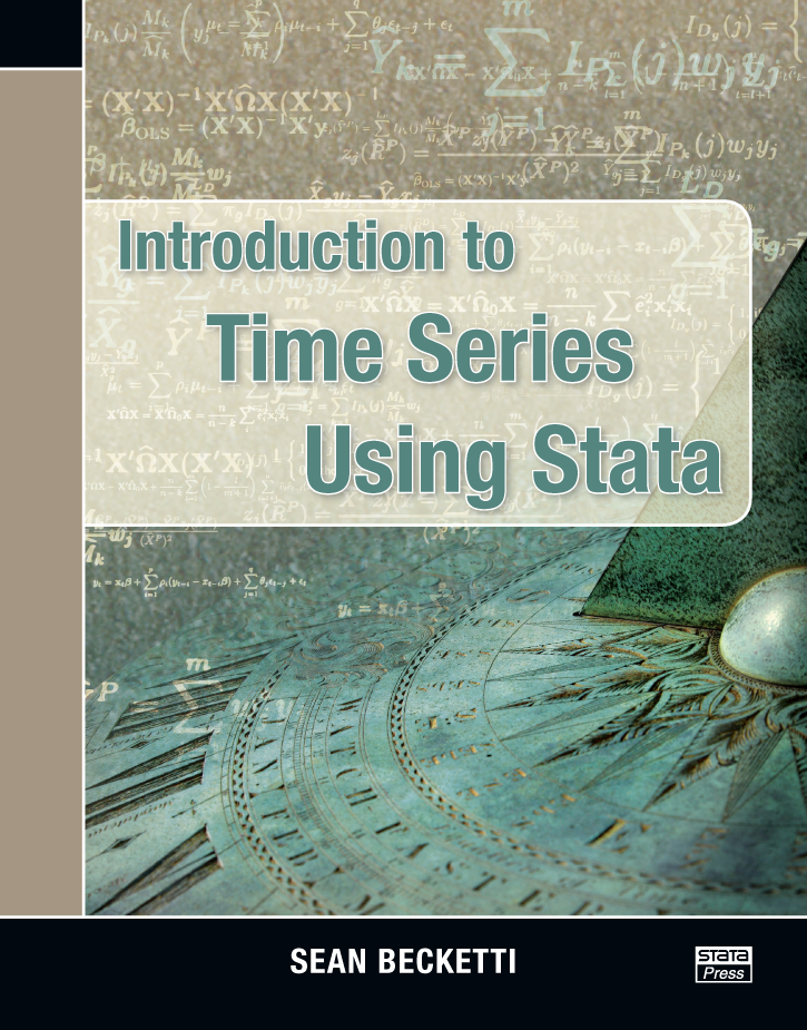
An Introduction to Times Series Analysis Using Stata - By Sean Becketti

Introduction to Time Series Using Stata, by Sean Becketti, provides a practical guide to working with time-series data using Stata and will appeal to a broad range of users. The many examples, concise explanations that focus on intuition, and useful tips based on the author’s decades of experience using time-series methods make the book insightful not just for academic users but also for practitioners in industry and government.

The book is appropriate both for new Stata users and for experienced users who are new to time-series analysis.

Chapter 1 provides a mild yet fast-paced introduction to Stata, highlighting all the features a user needs to know to get started using Stata for time-series analysis. Chapter 2 is a quick refresher on regression and hypothesis testing, and it defines key concepts such as white noise, autocorrelation, and lag operators.

Chapter 3 begins the discussion of time series, using moving-average and Holt–Winters techniques to smooth and forecast the data. Becketti also introduces the concepts of trends, cyclicality, and seasonality and shows how they can be extracted from a series. Chapter 4 focuses on using these methods for forecasting and illustrates how the assumptions regarding trends and cycles underlying the various moving-average and Holt–Winters techniques affect the forecasts produced. Although these techniques are sometimes neglected in other time-series books, they are easy to implement, can be applied to many series quickly, often produce forecasts just as good as more complicated techniques, and as Becketti emphasizes, have the distinct advantage of being easily explained to colleagues and policy makers without backgrounds in statistics.

Chapters 5 through 8 encompass single-equation time-series models. Chapter 5 focuses on regression analysis in the presence of autocorrelated disturbances and details various approaches that can be used when all the regressors are strictly exogenous but the errors are autocorrelated, when the set of regressors includes a lagged dependent variable and independent errors, and when the set of regressors includes a lagged dependent variable and autocorrelated errors. Chapter 6 describes the ARIMA model and Box–Jenkins methodology, and chapter 7 applies those techniques to develop an ARIMA-based model of U.S. GDP. Chapter 7 in particular will appeal to practitioners because it goes step by step through a real-world example: here is my series, now how do I fit an ARIMA model to it? Chapter 8 is a self-contained summary of ARCH/GARCH modeling.

In the final portion of the book, Becketti discusses multiple-equation models, particularly VARs and VECs. Chapter 9 focuses on VAR models and illustrates all key concepts, including model specification, Granger causality, impulse-response analyses, and forecasting, using a simple model of the U.S. economy; structural VAR models are illustrated by imposing a Taylor rule on interest rates. Chapter 10 presents nonstationary time-series analysis. After describing nonstationarity and unit-root tests, Becketti masterfully navigates the reader through the often-confusing task of specifying a VEC model, using an example based on construction wages in Washington, DC, and surrounding states. Chapter 11 concludes.

Sean Becketti is a financial industry veteran with three decades of experience in academics, government, and private industry. He was a developer of Stata in its infancy, and he was Editor of the Stata Technical Bulletin, the precursor to the Stata Journal, between 1993 and 1996. He has been a regular Stata user since its inception, and he wrote many of the first time-series commands in Stata.

Introduction to Time Series Using Stata, by Sean Becketti, is a first-rate, example-based guide to time-series analysis and forecasting using Stata. It can serve as both a reference for practitioners and a supplemental textbook for students in applied statistics courses.

1. Just enough Stata
   1.1 Getting started 
   

   1.1.1 Action first, explanation later 
   1.1.2 Now some explanation 
   1.1.3 Navigating the interface 
   1.1.4 The gestalt of Stata 
   1.1.5 The parts of Stata speech 
   

   1.2 All about data 
   1.3 Looking at data 
   1.4 Statistics 
   

   1.4.1 Basics 
   1.4.2 Estimation 
   

   1.5 Odds and ends 
   1.6 Making a date 
   

   1.6.1 How to look good 
   1.6.2 Transformers 
   

   1.7 Typing dates and date variables 
   1.8 Looking ahead 
   
   2 Just enough statistics
   2.1 Random variables and their moments 
   2.2 Hypothesis tests 
   2.3 Linear regression 
   

   2.3.1 Ordinary least squares 
   2.3.2 Instrumental variables 
   2.3.3 FGLS 
   

   2.4 Multiple-equation models 
   2.5 Time series 
   

   2.5.1 White noise, autocorrelation, and stationarity 
   2.5.2 ARMA models 
   
   3 Filtering time-series data
   3.1 Preparing to analyze a time series 
   

   3.1.1 Questions for all types of data 
   

   How are the variables defined? 
   What is the relationship between the data and the phenomenon of interest? 
   Who compiled the data? 
   What processes generated the data? 
   

   3.1.2 Questions specifically for time-series data 
   

   What is the frequency of measurement? 
   Are the data seasonally adjusted? 
   Are the data revised? 
   

   3.2 The four components of a time series 
   

   Trend 
   Cycle 
   Seasonal 
   

   3.3 Some simple filters 
   

   3.3.1 Smoothing a trend 
   3.3.2 Smoothing a cycle 
   3.3.3 Smoothing a seasonal pattern 
   3.3.4 Smoothing real data 
   

   3.4 Additional filters 
   

   3.4.1 ma: Weighted moving averages 
   3.4.2 EWMAs 
   

   exponential: EWMAs 
   dexponential: Double-exponential moving averages 
   

   3.4.3 Holt–Winters smoothers 
   

   hwinters: Holt–Winters smoothers without a seasonal component 
   shwinters: Holt–Winters smoothers including a seasonal component 
   

   3.5 Points to remember 
   
   4 A first pass at forecasting
   4.1 Forecast fundamentals 
   

   4.1.1 Types of forecasts 
   4.1.2 Measuring the quality of a forecast 
   4.1.3 Elements of a forecast 
   

   4.2 Filters that forecast 
   

   4.2.1 Forecasts based on EWMAs 
   4.2.2 Forecasting a trending series with a seasonal component 
   

   4.3 Points to remember 
   4.4 Looking ahead 
   
   5 Autocorrelated disturbances
   5.1 Autocorrelation 
   

   5.1.1 Example: Mortgage rates 
   

   5.2 Regression models with autocorrelated disturbances 
   

   5.2.1 First-order autocorrelation 
   5.2.2 Example: Mortgage rates (cont.) 
   

   5.3 Testing for autocorrelation 
   

   5.3.1 Other tests 
   

   5.4 Estimation with first-order autocorrelated data 
   

   5.4.1 Model 1: Strictly exogenous regressors and autocorrelated disturbances 
   

   The OLS strategy 
   The transformation strategy 
   The FGLS strategy 
   Comparison of estimates of model 
   

   5.4.2 Model 2: A lagged dependent variable and i.i.d. errors 
   5.4.3 Model 3: A lagged dependent variable with AR(1) errors 
   

   The transformation strategy 
   The IV strategy 
   

   5.5 Estimating the mortgage rate equation 
   5.6 Points to remember 
   
   6 Univariate time-series models
   6.1 The general linear process 
   6.2 Lag polynomials: Notation or prestidigitation? 
   6.3 The ARMA model 
   6.4 Stationarity and invertibility 
   6.5 What can ARMA models do? 
   6.6 Points to remember 
   6.7 Looking ahead 
   
   7 Modeling a real-world time series
   7.1 Getting ready to model a time series 
   7.2 The Box–Jenkins approach 
   7.3 Specifying an ARMA model 
   

   7.3.1 Step 1: Induce stationarity (ARMA becomes ARIMA) 
   7.3.2 Step 2: Mind your p’s and q’s 
   

   7.4 Estimation 
   7.5 Looking for trouble: Model diagnostic checking 
   

   7.5.1 Overfitting 
   7.5.2 Tests of the residuals 
   

   7.6 Forecasting with ARIMA models 
   7.7 Comparing forecasts 
   7.8 Points to remember 
   7.9 What have we learned so far? 
   7.10 Looking ahead 
   
   8 Time-varying volatility
   8.1 Examples of time-varying volatility 
   8.2 ARCH: A model of time-varying volatility 
   8.3 Extensions to the ARCH model 
   

   8.3.1 GARCH: Limiting the order of the model 
   8.3.2 Other extensions 
   

   Asymmetric responses to “news” 
   Variations in volatility affect the mean of the observable series 
   Nonnormal errors 
   Odds and ends 
   

   8.4 Points to remember 
   
   9 Models of multiple time series
   9.1 Vector autoregressions 
   

   9.1.1 Three types of VARs 
   

   9.2 A VAR of the U.S. macroeconomy 
   

   9.2.1 Using Stata to estimate a reduced-form VAR 
   9.2.2 Testing a VAR for stationarity 
   

   Other tests 
   

   9.2.3 Forecasting 
   

   Evaluating a VAR forecast 
   

   9.3 Who’s on first? 
   

   9.3.1 Cross correlations 
   9.3.2 Summarizing temporal relationships in a VAR 
   

   Granger causality 
   How to impose order 
   FEVDs 
   Using Stata to calculate IRFs and FEVDs 
   

   9.4 SVARs 
   

   9.4.1 Examples of a short-run SVAR 
   9.4.2 Examples of a long-run SVAR 
   

   9.5 Points to remember 
   9.6 Looking ahead 
   
   10 Models of nonstationary time series
   10.1 Trends and unit roots 
   10.2 Testing for unit roots 
   10.3 Cointegration: Looking for a long-term relationship 
   10.4 Cointegrating relationships and VECMs 
   10.4.1 Deterministic components in the VECM 
   10.5 From intuition to VECM: An example 
   

   Step 1: Confirm the unit root 
   Step 2: Identify the number of lags 
   Step 3: Identify the number of cointegrating relationships 
   Step 4: Fit a VECM 
   Step 5: Test for stability and white-noise residuals 
   Step 6: Review the model implications for reasonableness 
   

   10.6 Points to remember 
   10.7 Looking ahead 
   
   11 Closing observations
   11.1 Making sense of it all 
   11.2 What did we miss? 
   

   11.2.1 Advanced time-series topics 
   11.2.2 Additional Stata time-series features 
   

   Data management tools and utilities 
   Univariate models 
   Multivariate models 
   

   11.3 Farewell

References
Author Index
Subject Index

© Copyright StataCorp LP 2002-2013.