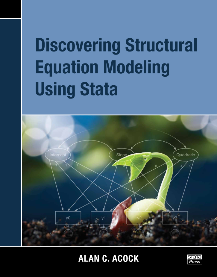
Discovering Structural Equation Modeling Using Stata

di Alan Acock

 Discovering Structural Equation Modeling Using Stata, by Alan Acock, successfully introduces both the statistical principles involved in structural equation modeling (SEM) and the use of Stata to fit these models. The book uses an application-based approach to teaching SEM. Acock demonstrates how to fit a wide variety of models that fall within the SEM framework and provides datasets that enable the reader to follow along with each example. As each type of model is discussed, concepts such as identification, handling of missing data, model evaluation, and interpretation are covered in detail.

In Stata, structural equation models can be fit using the command language or the graphical user interface (GUI) for SEM, known as the SEM Builder. The book demonstrates both of these approaches. Throughout the text, the examples use the sem command. Each chapter also includes brief discussions on drawing the appropriate path diagram and performing estimation from in the SEM builder. A more in-depth coverage of the SEM Builder is given in one of the book’s appendixes.

The first two chapters introduce the building blocks of SEM. Chapter 1 begins with overviews of Chronbach’s alpha as a measure of reliability and of exploratory factor analysis. Then, building on these concepts, Acock demonstrates how to perform confirmatory factor analysis, discusses a variety of statistics available for assessing the fit of the model, and shows a more general measurement of reliability that is based on confirmatory factor analysis. Chapter 2 focuses on using SEM to perform path analysis. It includes examples of mediation, moderation, cross-lagged panel models, and nonrecursive models.

Chapter 3 demonstrates how to combine the topics covered in the first two chapters to fit full structural equation models. The use of modification indices to guide model modification and computation of direct, indirect, and total effects for full structural equation models are also covered.

Chapter 4 details the application of SEM to growth curve modeling. After introducing the basic linear latent growth curve model, Acock extends this to more complex cases such as the inclusion of quadratic terms, time-varying covariates, and time-invariant covariates.

Chapter 5 discusses testing for differences across groups in SEM. The author introduces the specialized sem syntax for multiple group models and discusses the intricacies of testing for group differences for the different types of models presented in the preceding chapters.

Discovering Structural Modeling Using Stata is an excellent resource both for those who are new to SEM and for those who are familiar with SEM but new to fitting these models in Stata. It is useful as a text for courses covering SEM as well as for researchers performing SEM.

Table of contents

List of Tables

List of Figures

List of examples

Preface

Acknowledgements

1 Introduction to confirmatory factor analysis

1.1 Introduction

1.2 The "do not even think about it" approach

1.3 The principal component factor analysis approach

1.4 Alpha reliability for our nine-item scale
1.5 Generating a factor score rather than a mean or summative score
1.6 What can CFA add?
1.7 Fitting a CFA model
1.8 Interpreting and presenting CFA results
1.9 Assessing goodness of fit
         1.9.1 Modification indices
         1.9.2 Final model and estimating scale reliability
1.10 A two-factor model
         1.10.1 Evaluating the depression dimension
         1.10.2 Estimating a two-factor model

1.11 Parceling
1.12 Extensions and what is next
1.13 Exercises
1.A Using the SEM Builder to run a CFA
         1.A.1 Drawing the model
         1.A.2 Estimating the model  

2 Using structural equation modeling for path models

2.1 Introduction
2.2 Path model terminology
        2.2.1 Exogenous predictor, endogenous outcome, and endogenous mediator   variables
        2.2.2 A hypothetical path model
2.3 A substantive example of a path model
2.4 Estimating a model with correlated residuals

        2.4.1 Estimating direct, indirect, and total effects
        2.4.2 Strengthening our path model and adding covariates
2.5 Auxiliary variables
2.6 Testing equality of coefficients
2.7 A cross-lagged panel design
2.8 Moderation
2.9 Nonrecursive models
         2.9.1 Worked example of a nonrecursive model
         2.9.2 Stability of a nonrecursive model
         2.9.3 Model constraints
         2.9.4 Equality constraints
2.10 Exercises
2.B Using the SEM Builder to run path models
The probit model

3 Structural equation modeling

3.1 Introduction
3.2 The classic example of a structural equation model
         3.2.1 Identification of a full structural equation model
         3.2.2 Fitting a full structural equation model
         3.2.3 Modifying our model
         3.2.4 Indirect effects
3.3 Equality constraints
3.4 Programming constraints
3.5 Structural model with formative indicators
         3.5.1 Identification and estimation of a composite latent variable
         3.5.2 Multiple indicators, multiple causes model
3.6 Exercises

4 Latent growth curves

5 Group comparisons

5.1 Interaction as a traditional approach to multiple-group comparisons
5.2 The range of applications of Stata’s multiple-group comparisons with sem
         5.2.1 A multiple indicators, multiple causes model
         5.2.2 A measurement model
         5.2.3 A full structural equation model
5.3 A measurement model application
         5.3.1 Step 1: Testing for invariance comparing women and men
         5.3.2 Step 2: Testing for invariant loadings
         5.3.3 Step 3: Testing for an equal loadings and equal errorvariances model
         5.3.4 Testing for equal intercepts
         5.3.5 Comparison of models
         5.3.6 Step 4: Comparison of means
         5.3.7 Step 5: Comparison of variances and covariance of latent variables
5.4 Multiple-group path analysis
         5.4.1 What parameters are different?
         5.4.2 Fitting the model with the SEM Builder
         5.4.3 A standardized solution
         5.4.4 Constructing tables for publications
5.5 Multiple-group comparisons of structural equation models
5.6 Exercises

6 Epilogue—what now?

A The graphical user interface

A.1 Introduction
A.2 Menus for Windows, Unix, and Mac
         A.2.1 The menus, explained
         A.2.2 The vertical drawing toolbar
A.3 Designing a structural equation model
A.4 Drawing an SEM model
A.5 Fitting a structural equation model
A.6 Postestimation commands
A.7 Clearing preferences and restoring the defaults

B Entering data from summary statistics

References

Author Index

Subject Index

© Copyright StataCorp LP 2002-2013.