| |
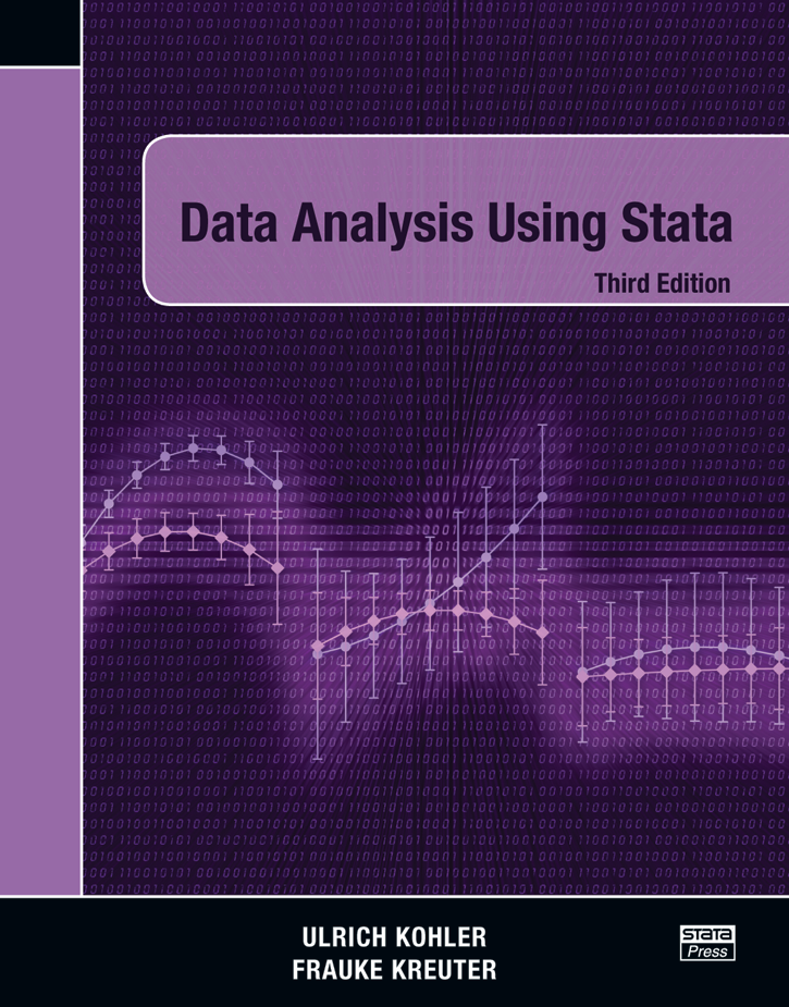
Data Analysis Using Stata, Third Edition - By Ulrich Kohler and Frauke Kreuter Comment from the Stata Technical group
 Data
Analysis Using Stata, Third Edition has been completely revamped to
reflect the capabilities of Stata 12. This book will appeal to those
just learning statistics and Stata, as well as to the many users who
are switching to Stata from other packages. Throughout the book, Kohler
and Kreuter show examples using data from the German Socio-Economic
Panel, a large survey of households containing demographic, income,
employment, and other key information. Data
Analysis Using Stata, Third Edition has been completely revamped to
reflect the capabilities of Stata 12. This book will appeal to those
just learning statistics and Stata, as well as to the many users who
are switching to Stata from other packages. Throughout the book, Kohler
and Kreuter show examples using data from the German Socio-Economic
Panel, a large survey of households containing demographic, income,
employment, and other key information.
Kohler and Kreuter take a hands-on approach, first showing how to use
Stata’s graphical interface and then describing Stata’s syntax. The
core of the book covers all aspects of social science research,
including data manipulation, production of tables and graphs, linear
regression analysis, and logistic modeling. The authors describe
Stata’s handling of categorical covariates and show how the new margins
and marginsplot commands greatly simplify the interpretation of
regression and logistic results. An entirely new chapter discusses
aspects of statistical inference, including random samples, complex
survey samples, nonresponse, and causal inference.
The rest of the book includes chapters on reading text files into
Stata, writing programs and do-files, and using Internet resources such
as the search command and the SSC archive.
Data Analysis Using Stata, Third Edition has been structured so that it
can be used as a self-study course or as a textbook in an introductory
data analysis or statistics course. It will appeal to students and
academic researchers in all the social sciences.
Table of Contents
List of Tables
List of Figures
Preface
- "The first time"
- 1.1 Starting Stata
- 1.2 Setting up your screen
- 1.3 Your first analysis
- 1.3.1 Inputting commands
- 1.3.2 Files and the working memory
- 1.3.3 Loading data
- 1.3.4 Variables and observations
- 1.3.5 Looking at data
- 1.3.6 Interrupting a command and repeating a command
- 1.3.7 The variable list
- 1.3.8 The in qualifier
- 1.3.9 Summary statistics
- 1.3.10 The if qualifier
- 1.3.11 Define missing values
- 1.3.12 The by prefix
- 1.3.13 Command options
- 1.3.14 Frequency tables
- 1.3.15 Graphs
- 1.3.16 Getting help
- 1.3.17 Recoding of variables
- 1.3.18 Variable labels and value labels
- 1.3.19 Linear regression
- 1.4 Do-files
- 1.5 Exiting Stata
- 1.6 Exercises
- Working with do-files
- 2.1 From interactive work to working with a do-file
- 2.1.1 Alternative 1
- 2.1.2 Alternative 2
- 2.2 Designing do-files
- 2.2.1 Comments
- 2.2.2 Line breaks
- 2.2.3 Some crucial commands
- 2.3 Organizing your work
- 2.4 Exercises
- The grammar of Stata
- 3.1 The elements of Stata commands
- 3.1.1. Stata commands
- 3.1.2 The variable list
- List of variables: required or optionals
- Abbreviation rules
- Special listings
- 3.1.3 Options
- 3.1.4 The in qualifier
- 3.1.5 The if qualifier
- 3.1.6 Expressions
- Operators
- Functions
- 3.1.7 Lists of numbers
- 3.1.8 Using filenames
- 3.2 Repeating similar commands
- 3.2.1 The by prefix
- 3.2.2 The foreach loop
- The types of foreach lists
- Several commands within a foreach loop
- 3.2.3 The forvalues loop
- 3.3 Weights
- Frequency weights
- Analytic weights
- Probability weights
- 3.4 Exercises
- General comments on the statistical commands
- 4.1 Regular statistical commands
- 4.2 Estimation commands
- 4.3 Exercises
- Creating and changing variables
- 5.1 The commands generate and replace
- 5.1.1 Variable names
- 5.1.2 Some examples
- 5.1.3 Useful functions
- 5.1.4 Changing codes with by, n, and N
- 5.1.5 Subscripts
- 5.2 Specialized recoding commands
- 5.2.1 The recode command
- 5.2.2 The egen command
- 5.3 Recording string variables
- 5.4 Recording date and time
- 5.4.1 Dates
- 5.4.2 Time
- 5.5 Setting missing values
- 5.6 Labels
- 5.7 Storage types, or, the ghost in the machine
- 5.8 Exercises
- Creating and changing graphs
- 6.1 A primer on graph syntax
- 6.2 Graph types
- 6.2.1 Examples
- 6.2.2 Specialized graphs
- 6.3 Graph elements
- 6.3.1 Appearance of data
- Choice of marker
- Marker colors
- Marker size
- Lines
- 6.3.2 Graphs and plot regions
- Graph size
- Plot region
- Scaling the axes
- 6.3.3 Information inside the plot region
- Reference lines
- Labeling inside the plot region
- 6.3.4 Information outside the plot region
- Labeling the axes
- Tick lines
- Axis titles
- The legend
- Graph titles
- 6.4 Multiple graphs
- 6.4.1 Overlaying numerous twoway graphs
- 6.4.2 Option by()
- 6.4.3 Combining graphs
- 6.5 Saving and printing graphs
- 6.6 Exercises
- Describing and Comparing Distributions
- 7.1 Categories: Few or many?
- 7.2 Variables with few categories
- 7.2.1 Tables
- Frequency tables
- More than one frequency table
- Comparing distributions
- Summary statistics
- More than one contingency table
- 7.2.2 Graphs
- Histograms
- Bar charts
- Bar charts
- Dot chart
- 7.3 Variables with many categories
- 7.3.1 Frequencies of grouped data
- Some remarks on grouping data
- Special techniques for grouping data
- 7.3.2 Describing data using statistics
- Important summary statistics
- The summarize command
- The tabstat command
- Comparing distributions using statistics
- 7.3.3 Graphs
- Box plots
- Histograms
- Kernel density estimation
- Quantile plot
- Comparing distributions with Q–Q plots
- 7.4 Exercises
- Statistical inference
8.1 Random samples and sampling distributions
8.1.1 Random numbers
8.1.2 Creating fictitious datasets
8.1.3 Drawing random samples
8.1.4 The sampling distribution
8.2 Descriptive inference
8.2.1 Standard errors for simple random samples
8.2.2 Standard errors for complex samples
Typical forms of complex samples
Sampling distributions for complex samples
Using Stata’s svy commands
8.2.3 Standard errors with nonresponse
Unit nonresponse and poststratification weights
Item nonresponse and multiple imputation
8.2.4 Uses of standard errors
Confidence intervals
Significance tests
Two-group mean comparison test
8.3 Causal inference
8.3.1 Basic concepts
Data-generating processes
Counterfactual concept of causality
8.3.2 The effect of third-class tickets
8.3.3 Some problems of causal inference
8.4 Exercises
9. Introduction to linear regression
- 9.1 Simple linear regression
- 9.1.1 The basic principle
- 9.1.2 Linear regression using Stata
- The table of coefficients
- Standard errors
- The table of ANOVA results
- The model fit table
- 9.2 Multiple regression
- 9.2.1 Multiple regression using Stata
- 9.2.2 Additional components
- Adjusted R2
- Standardized regression coefficients
- 9.2.3 What does "under control" mean?
- 9.3 Regression diagnostics
- 9.3.1 Violation of E(εi) = 0
- Linearity
- Influential cases
- Omitted variables
- Multicollinearity
- 9.3.2 Violation of Var(εi) = σ2
- 9.3.3 Violation of Cov(εi, εj) = 0, i ≠ j
- 9.4 Model extensions
- 9.4.1 Categorical independent variables
- 9.4.2 Interaction terms
- 9.4.3 Regression models using transformed variables
- Nonlinear relations
- Eliminating heteroskedasticity
- 9.5 Reporting regression results
9.5.1 Tables of similar regression models
9.5.2 Plots of coefficients
9.5.3 Conditional-effects plots
- 9.6 Advanced techniques
- 9.6.1 Median regression
- 9.6.2 Regression models for panel data
- From wide to long format
- Fixed-effects models
- 9.6.3 Error-component models
- 9.7 Exercises
- Regression models for Categorical Dependent Variables
- 10.1 The linear probability model
- 10.2 Basic concepts
- 9.2.1 Odds, log odds, and odds ratios
- 9.2.2 Excursion: The maximum likelihood principle
- 10.3 Logistic regression with Stata
- 10.3.1 The coefficients table
- Sign interpretation
- Interpretation with odds ratios
- Probability interpretation
- Average marginal effects
- 10.3.2 The iteration block
- 10.3.3 The model fit block
- Classification tables
- Pearson chi-squared
- 10.4 Logistic regression diagnostics
- 9.4.1 Linearity
- 9.4.2 Influential cases
- 10.5 Likelihood-ratio test
- 10.6 Refined models
- 10.6.1 Nonlinear relationships
- 10.6.2 Interaction effects
- 10.7 Advanced techniques
- 10.7.1 Probit models
- 10.7.2 Multinomial logistic regression
- 10.7.3 Models for ordinal data
- 10.8 Exercises
- Reading and writing data
- 11.1 The goal: The data matrix
- 11.2 Importing machine-readable data
- 11.2.1 Reading system files from other packages
-
Reading Excel files
Reading SAS transport files
Reading other system files
- 11.2.2 Reading ASCII text files
- Reading data in spreadsheet format
- Reading data in free format
- Reading data in fixed format
- 11.3 Inputting data
- 11.3.1 Input data using the editor
- 11.3.2 The input command
- 11.4 Combining data
- 11.4.1 The GSOEP database
- 11.4.2 The merge command
- Merge 1:1 matches with rectangular data
- Merge 1:1 matches with nonrectangular data
- Merging more than two files
- Merging m:1 and 1:m matches
- 11.4.3 The append command
- 11.5 Saving and exporting data
- 11.6 Handling lage datasets
- 10.6.1 Rules for handling the working memory
- 10.6.2 Using oversized datasets
- 11.7 Exercises
- Do-files for advanced users and user-written programs
- 12.1 Two examples of usage
- 12.2 Four programming tools
- 12.2.1 Local macros
- Calculating with local macros
- Combining local macros
- Changing local macros
- 12.2.2 Do-files
- 12.2.3 Programs
- The problem of redefinition
- The problem of naming
- The problem of error checking
- 12.2.4 Programs in do-files and ado-files
- 12.3 User-written Stata commands
-
- 12.3.1 12.3.1 Sketch of the syntax
12.3.2 Create a first ado-file
- 12.3.3 Parsing variable lists
- 11.3.4 Parsing options
- 11.3.5 Parsing if and in qualifiers
- 11.3.6 Generating an unknown number of variables
- 11.3.7 Default values
- 11.3.8 Extended macro functions
- 11.3.9 Avoiding changes in the dataset
- 11.3.10 Help files
- 12.4 Exercises
- Around Stata
- 13.1 Resources and information
- 13.2 Taking care of Stata
- 13.3 Additional procedures
- 13.3.1 Stata Journal ado-files
- 13.3.2 SSC ado-files
- 13.3.3 Other ado-files
- 13.4 Exercises
References
Authors Index
Subject Index
© Copyright StataCorp LP 2002-2010.


|
|


